Damien Mannion

Data are sometimes on a circular scale (also known as directional), and circular data often need to be analysed differently to non-circular data. In perception research, this often occurs with things like stimulus orientation and camera rotations—where the measurement is in angles. A classic example of the need for specialised analysis methods is where we have a pair of angles, say 300° and 10°, and we would like to calculate the mean. Using the typical calculation for the mean gives 155°, which is not a good measure of the central tendency of this data. Instead, we can use the circular mean (via scipy.stats.circmean, for example), which gives 335°.

Two probability distributions that are suitable for use with circular data are the wrapped normal distribution and the von Mises distribution. The distributions are similar, and we will focus here on the von Mises distribution because it is implemented in PyMC. Here, we will look at how we can fit a von Mises distribution to some circular data in PyMC.

Generating the example data

We generate some example data using the method for generating random values from a specified von Mises distribution in numpy. Here, we will set the mean parameter (μ) to 135° and the standard deviation parameter (σ) to 45° and draw 100 random values.

rand = np.random.default_rng(seed=21056627)

n_obs = 100

mu = np.radians(135)
sigma = np.radians(45)
kappa = 1 / (sigma ** 2)

data = rand.vonmises(mu=mu, kappa=kappa, size=n_obs)

Note that the distribution in numpy is parameterised by κ (kappa), which is the inverse of the variance. It also requires the parameters to be specified in radians and produces values in the range of [−π, +π].

A histogram of these values is shown below. Note how the values ‘wrap around’, and how this can make our distribution appear to be bimodal if we are not aware that it is circular data.

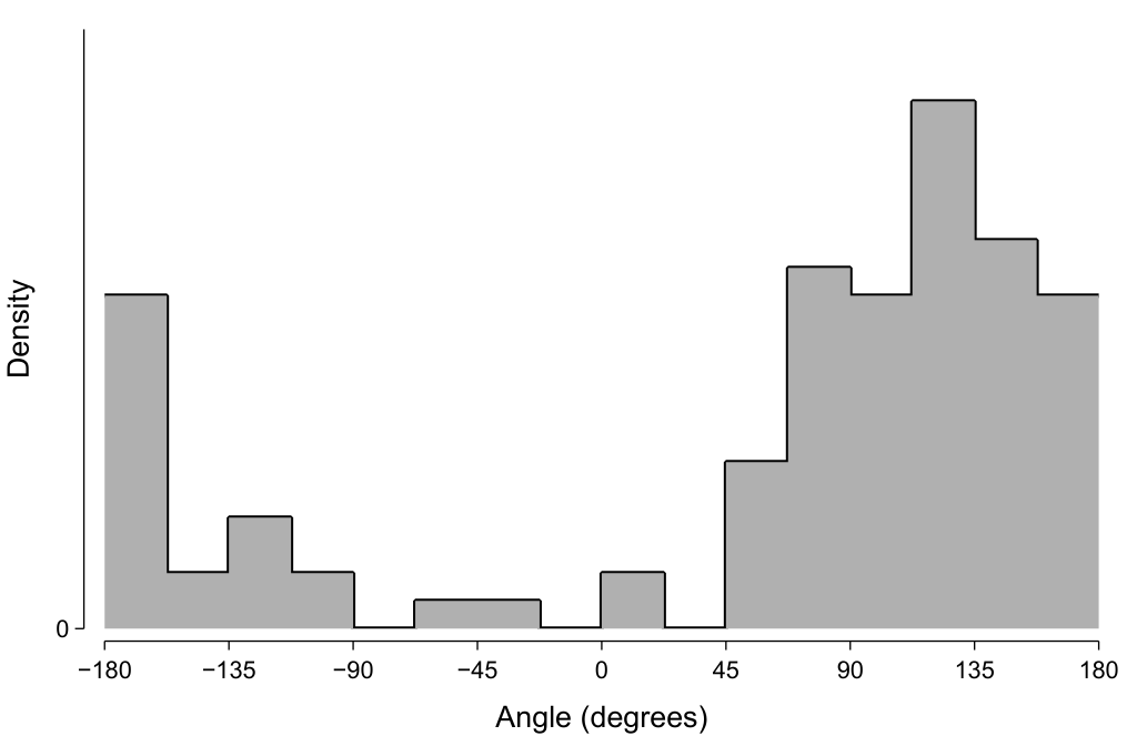
Should this histogram be plotted on polar rather than Cartesian axes? Polar axes do indeed seem well-suited, given that they are specified by angle and length—which matches the characteristics of this plotted data. However, I find graphs using polar axes to be more difficult to visually understand and so I tend to prefer using Cartesian axes. Sometimes it is useful to add a redundant quarter-cycle or so to the left and right edges to make the circularity more evident and not ‘disadvantage’ the data at the boundaries.

Specifying the model

Our goal now is to fit a model to this observed data and estimate the parameters of the distribution from which it was generated. Within the Bayesian framework, this involves placing priors on the unknown parameters—here, μ and σ. The details of the priors need to be specific to the particular circumstances of a given analysis, and pm.sample_prior_predictive can be very useful in visualising the consequences of the selected prior values to check that they align with the intentions.

Here, we will use a uniform prior for μ, expressing our prior belief that the parameter could be anywhere within the circular range. Importantly, we need to indicate the circularity of this μ parameter to pymc by using the transform argument when specifying the prior distribution. We will use a broad half-normal distribution for the standard deviation.

This model can be implemented in pymc via:

with pm.Model() as model:

    mu = pm.Uniform(
        "mu",
        lower=-np.pi,
        upper=+np.pi,
        transform=pm.transforms.Circular(),
    )

    sigma = pm.HalfNormal("sigma", sigma=np.radians(90))

    kappa = 1 / (sigma ** 2)

    pm.VonMises(
        "obs",
        mu=mu,
        kappa=kappa,
        observed=data,
    )

More complex models are sometimes necessary to incorporate the presence of bimodality within the circular data, such as using a pm.Mixture distribution. This bimodality can sometimes occur at 180° separations, which can provide some additional information to constrain the priors. However, ‘label switching’ (Jasra, Holmes, & Stephens, 2005) can be an issue with circular data in particular (Mulder, Jongsma, & Klugkist, 2020) and can require additional consideration.

Sampling and model evaluation

We can run the MCMC sampling process using pymc via:

with model:
    idata = pm.sample(return_inferencedata=True)

I am using return_inferencedata=True so that the result of the sampling process is an arviz (Kumar, Carroll, Hartikainen, & Martin, 2019) InferenceData object, which is not the default in pymc3 (which I am using here)—but it will become the default in the upcoming release of pymc. I was slow to come around to the benefits of the InferenceData representation, but I have since become a big fan of xarray (Hoyer & Hamman, 2017), upon which InferenceData is based, and now prefer this sort of representation in most of my programming.

It is important to note that the posterior samples for μ are also circular data, so we need to be careful with how they are summarised. Happily, arviz is able to appropriately deal with circular data in many instances. For example, obtaining the mean of the posterior using az.summary can use the circular mean if the argument circ_var_names=["mu"] is provided. Doing so here gives a mean of about 132.75°, which is close to the value of μ in the generating distribution (135°).

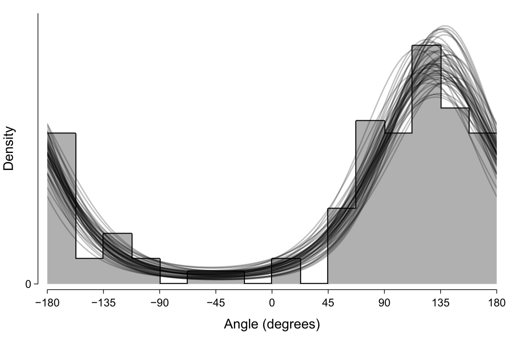
One way we can evaluate the descriptive adequacy of the model is to randomly draw samples from the fitted posterior (here, μ and σ) and use those to evaluate the probability density function at a range of angles. As expected, the 50 such samples shown in the below depict distributions that appear to visually approximate the histogram of the observed data.

Summary

Circular data often need to be analysed using specialised procedures that take the circularity into account. Here, we looked at how we can use PyMC to fit a simple model to some circular data.

Software versions

Here are the version of the key software and packages that were used to generate the material in this post:

Python implementation: CPython
Python version       : 3.9.12
IPython version      : 8.3.0

pymc3: 3.11.5
veusz: 3.4
numpy: 1.22.1
scipy: 1.7.3
arviz: 0.12.0

References

1. Hoyer, S. & Hamman, J. (2017) xarray: N-D labeled arrays and datasets in Python. Journal of Open Research Software, 5(1), 10–10.
2. Jasra, A., Holmes, C.C., & Stephens, D.A. (2005) Markov Chain Monte Carlo methods and the label switching problem in Bayesian mixture modeling. Statistical Science, 20(1), 50–67.
3. Kumar, R., Carroll, C., Hartikainen, A., & Martin, O. (2019) ArviZ: a unified library for exploratory analysis of Bayesian models in Python. Journal of Open Source Software, 4(33), 1143–1143.
4. Mulder, K., Jongsma, P., & Klugkist, I. (2020) Bayesian inference for mixtures of von Mises distributions using reversible jump MCMC sampler. Journal of Statistical Computation and Simulation, 90(9), 1539–1556.