Damien Mannion

Difference scaling is a model and experimental method outlined by Maloney & Yang (2003) for describing a stimulus dimension in terms of a psychophysical scale in which equal numerical differences are associated with equal perceptual differences.

Although they term their method “Maximum Likelihood Difference Scaling” (MLDS), here I will drop the “ML” part of it as I won’t be using maximum likelihood methods.

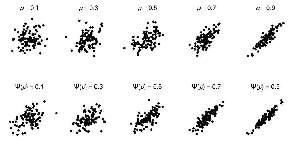
Knoblauch & Maloney (2008) give further details on the technique and its practical implementation. They also describe an example application of difference scaling concerning the visual perception of structure in scatterplots. Each panel in the figure below depicts 100 samples from a bivariate normal distribution with a covariance structure consistent with a particular population Pearson correlation coefficient (\(\rho\)). The aim in their example is to relate the stimulus scale (scatterplots depict draws from a distribution with a particular \(\rho\)) to a perceptual difference scale, and we will use their data to work through our own example.

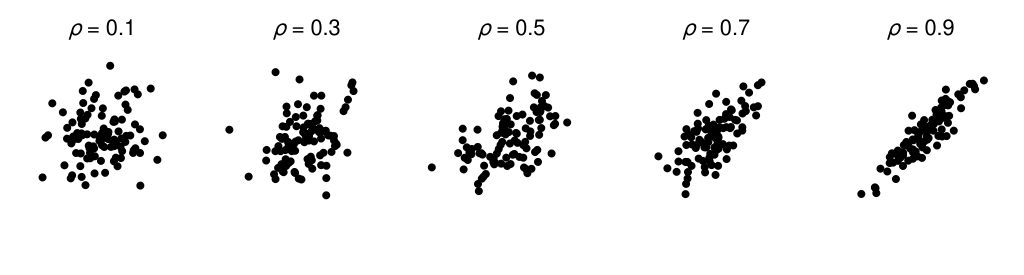
We won’t be going into some of the application-level subtleties that seem to be apparent with this particular example. For instance, the sample correlation coefficient for 100 pairs will be variable from draw-to-draw and hence won’t necessarily match the population correlation coefficient for a given draw.

Overview

Here, my goals are to:

• Describe the difference scaling method and work through the incorporation of a change to its assumptions.
• Implement a difference scaling model via Bayesian estimation procedures (using PyMC).
• Apply the method to the example scatterplot data provided by Knoblauch & Maloney (2008).

I will first describe my take on a general framework for difference scaling. I will then work through a model underlying the processing of a single trial within a difference scaling approach before describing a statistical model for multiple trials. I will then introduce parameter estimation in a Bayesian approach, giving particular attention to prior distributions. This approach will then be applied to the scatterplot example, before finishing with some additional considerations.

I will be using quite a few maths symbols and equations within the presentation below, which I hope is not discouraging. I am not strong in maths and I am trying to improve in my communication within that framework. Most of the concepts expressed in symbols and equations is also shown in Python code, which may offer a different route to understanding.

Framework

We begin by identifying the dimension for which we would like to estimate a perceptual scale, which we will refer to as \(x\). This dimension is numeric, ordered, and is assumed to be measured without error. In the example that we will be considering here, \(x\) is given by the population correlation coefficient (\(\rho\)) that generated the points shown in scatterplots. In other usages of similar methods, \(x\) has corresponded to things like specular reflectance (Sun & Mannion, 2021; Cheeseman, Ferwerda, Maile, & Fleming, 2021), image compression level (Charrier, Maloney, Cherifi, & Knoblauch, 2007), slant in depth (Aguilar, Wichmann, & Maertens, 2017), and chromatic magnitude (Kruse, Mannion, Alenin, & Tyo, 2022).

Our goal is to estimate a mapping from \(x\) to a representation in which equal numerical differences correspond to equal perceptual differences. This mapping forms our perceptual scale, and we will call it \(\Psi\) (“Psi”).

When an observer is presented with a stimulus with value \(x\) (e.g., a scatterplot depicting \(\rho = 0.4\)), we assume that their resulting internal response (\(y\)) relating to the dimension is given by the application of the perceptual scale (\(\Psi\)). However, we also assume that this response is stochastic, in that repeated presentations would not produce identical responses. We can describe this internal response as a draw from a normal distribution with a mean given by the evaluation of the perceptual scale at \(x\) and with the standard deviation (\(\sigma\)) capturing the variability: $$ y_x \sim \mathcal{N}\left(\Psi\left(x\right), \sigma\right). $$

Here, I am departing from the traditional treatment of difference scaling in which the variability is applied at a subsequent decision stage.

Trial model

In the difference scaling approach, a single trial consists of the presentation of two pairs of stimuli: \(\left(x_a, x_b\right)\) and \(\left(x_c, x_d\right)\). For example, one pair might be scatterplots depicting \(\left(\rho = 0.2, \rho = 0.4\right)\) and the other pair might be scatterplots depicting \(\left(\rho = 0.5, \rho = 0.9\right)\). In the typical “non-overlapping” implementation, these values are constrained such that \(x_a < x_b < x_c < x_d\).

As described previously, each of these stimuli is assumed to evoke an internal response that can be described as: $$ \begin{align*} y_a &\sim \mathcal{N}\left(\Psi\left(x_a\right), \sigma\right)\\ y_b &\sim \mathcal{N}\left(\Psi\left(x_b\right), \sigma\right)\\ y_c &\sim \mathcal{N}\left(\Psi\left(x_c\right), \sigma\right)\\ y_d &\sim \mathcal{N}\left(\Psi\left(x_d\right), \sigma\right). \end{align*} $$ Note that there are two assumptions about the variability that are being made here: that the variability is equal and that the variability is independent across stimuli.

The observer’s task is to judge whether the apparent perceptual difference is larger between \(\left(x_a, x_b\right)\) or between \(\left(x_c, x_d\right)\). We assume that, in undertaking this task, the observer calculates each pair’s signed perceptual difference (\(\delta\)): $$ \begin{align*} \delta_{ba} &= y_b - y_a\\ \delta_{dc} &= y_d - y_c. \end{align*} $$ Given our assumptions about \(y\), we can express this as: $$ \begin{align*} \delta_{ba} &\sim \mathcal{N}\left(\Psi\left(x_b\right) - \Psi\left(x_a\right), \sqrt{2}\sigma\right)\\ \delta_{dc} &\sim \mathcal{N}\left(\Psi\left(x_d\right) - \Psi\left(x_c\right), \sqrt{2}\sigma\right) \end{align*} $$

We can express \(\delta\) in this way because of the general equation for the difference of independent normal distributions: $$ \begin{align*} \mathcal{N}\left(x_1, \sigma\right) - \mathcal{N}\left(x_2, \sigma\right) &\sim \mathcal{N}\left(x_1 - x_2, \sqrt{\sigma^2 + \sigma^2}\right)\\ &\sim \mathcal{N}\left(x_1 - x_2, \sqrt{2\sigma^2}\right)\\ &\sim \mathcal{N}\left(x_1 - x_2, \sqrt{2}\sigma\right). \end{align*} $$

We assume that the observer then calculates the difference (\(\Delta\)) between the lengths (obtained by taking the absolute value) of these signed differences: $$ \Delta = \left|\delta_{dc}\right| - \left|\delta_{ba}\right|. $$ This then forms the basis for the binary decision (their response, \(r\)) regarding whether the perceptual difference between \(\left(x_c, x_d\right)\) was greater than (\(1\)) or less than (\(0\)) the perceptual difference between \(\left(x_a, x_b\right)\): $$ r = \begin{cases} 1 &\text{if } \Delta > 0\\ 0 &\text{if } \Delta < 0. \end{cases} $$

Now, we need to work out a way of expressing the probability of an observer’s response (\(r=0\) and \(r=1\)) given the set of trial components that we have considered: $$ \Set{x_a, x_b, x_c, x_d, \sigma, \Psi}. $$

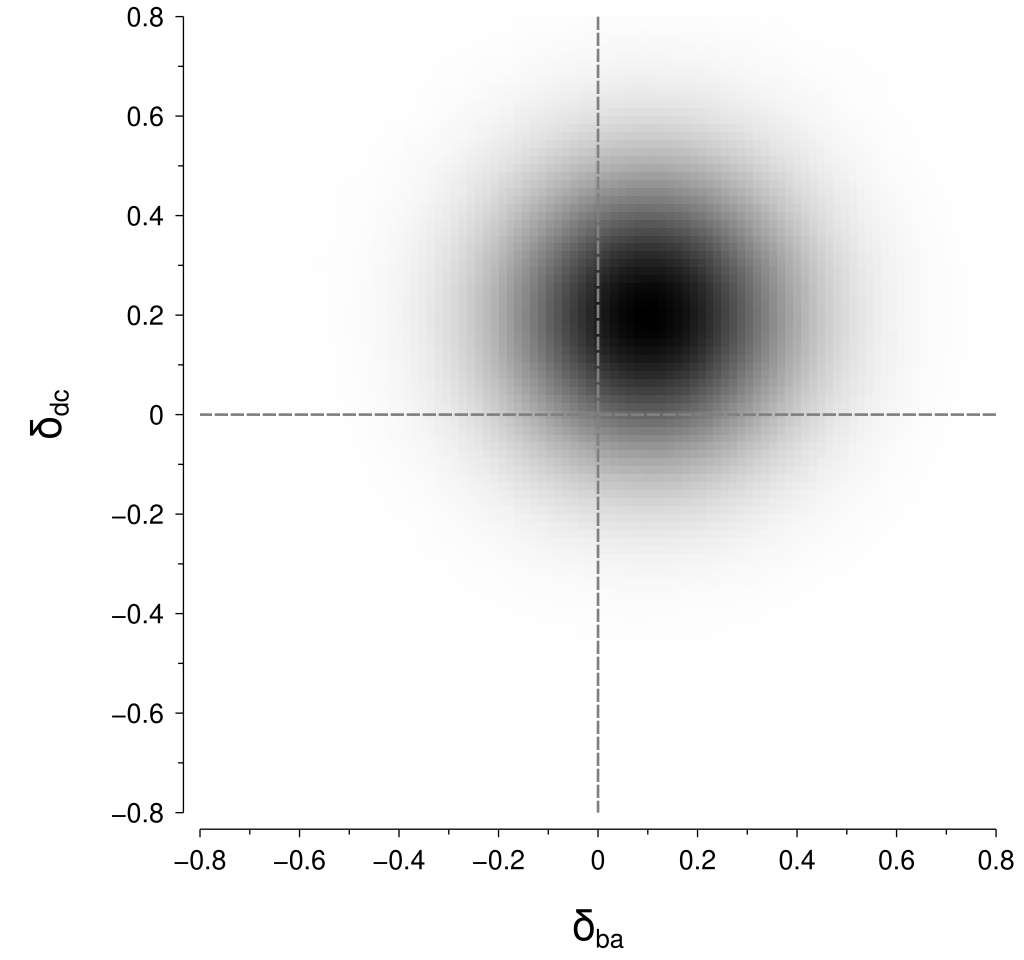
This gets a bit tricky with our new assumption of stimulus-level variability, mostly due to the absolute value operations in the length calculations. To understand this trickiness, it is helpful to inspect a visualisation for some example values; let’s specify some example values as: $$ \begin{align*} \Psi\left(x_b\right) - \Psi\left(x_a\right) = \mu_{ba} &= 0.1\\ \Psi\left(x_d\right) - \Psi\left(x_c\right) = \mu_{dc} &= 0.2\\ \sigma &= 0.14 \end{align*} $$ Now, we can visualise the joint probability density that corresponds to these example values as shown below:

To calculate the probability of the perceptual difference between \(\left(x_c, x_d\right)\) being greater than the perceptual difference between \(\left(x_a, x_b\right)\), we need to integrate within the regions in the above figure where \(\left|\delta_{dc}\right| > \left|\delta_{ba}\right|\). Those regions are highlighted in the figure below:

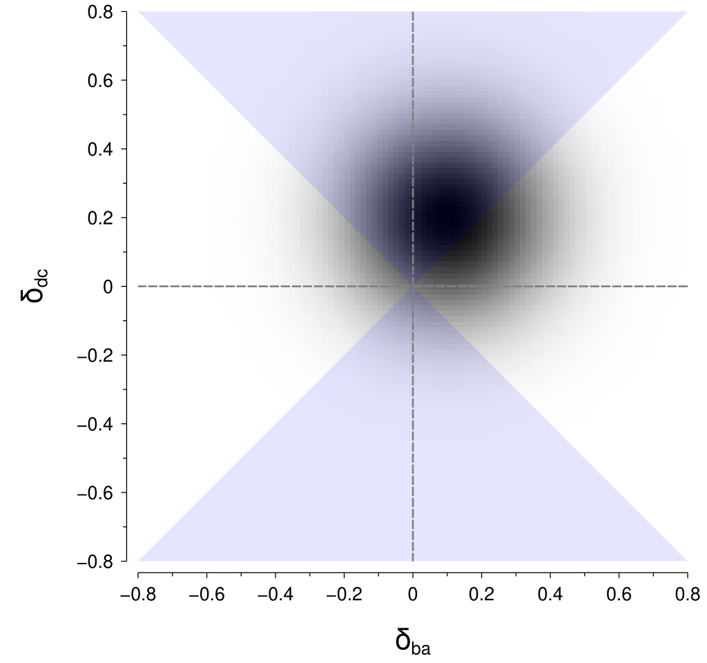
I don’t know of a good way to perform that computation for the particular geometry of those regions. However, there is a neat trick that we can use to put it into a form that is amenable to computation. By rotating the coordinates by 45° we obtain the rotated axes \(\delta_{ba}^\prime\) and \(\delta_{dc}^\prime\): $$ \begin{align*} \delta_{ba}^\prime &= \delta_{ba} \cos 45^\circ + \delta_{dc} \sin 45^\circ \\ \delta_{dc}^\prime &= -\delta_{ba} \sin 45^\circ + \delta_{dc} \cos 45^\circ. \end{align*} $$ Within these rotated coordinates, the means of our perceptual difference distributions are given by: $$ \begin{align*} \mu_{ba}^\prime &= \mu_{ba} \cos 45^\circ + \mu_{dc} \sin 45^\circ \\ \mu_{dc}^\prime &= -\mu_{ba} \sin 45^\circ + \mu_{dc} \cos 45^\circ \end{align*} $$ and their standard deviation (\(\sigma\)) is unchanged.

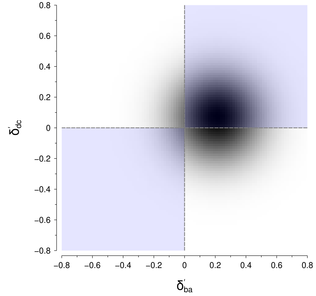
The nice thing about this rotation is that the regions now align nicely into quadrants, as shown below, for which we can integrate reasonably easily.

To calculate the probability in practice (i.e., in code), we first need a way of evaluating the cumulative distribution function (CDF) for a univariate normal distribution. Here, we will use the function from scipy and evaluate it at zero to give us the probability less than zero (ltz) for a given \(\left(\mu, \sigma\right)\) pair:

def norm_p_ltz(mu, sigma):
    return scipy.stats.norm.cdf(x=0.0, loc=mu, scale=sigma)

Second, we need a way of appropriately rotating our dimensions:

def rotate(x, y, rot_deg=45.0):

    rot_rad = np.radians(rot_deg)

    x_prime = x * np.cos(rot_rad) + y * np.sin(rot_rad)
    y_prime = -x * np.sin(rot_rad) + y * np.cos(rot_rad)

    return (x_prime, y_prime)

Now, we can define a psychometric function (pf) that implements the steps that have been described above:

def pf(mu, sigma, norm_p_ltz_func=norm_p_ltz):

    mu_a = mu[:, 0]
    mu_b = mu[:, 1]
    mu_c = mu[:, 2]
    mu_d = mu[:, 3]

    # signed differences
    ba_diff = mu_b - mu_a
    dc_diff = mu_d - mu_c

    # get 45 deg. rotated versions
    (ba_diff_prime, dc_diff_prime) = rotate(x=ba_diff, y=dc_diff)

    # use the CDF to calculate the probability below and above zero
    # for both dimensions
    p_rot_ba_ltz = norm_p_ltz_func(mu=ba_diff_prime, sigma=sigma)
    p_rot_ba_gtz = 1.0 - p_rot_ba_ltz
    p_rot_dc_ltz = norm_p_ltz_func(mu=dc_diff_prime, sigma=sigma)
    p_rot_dc_gtz = 1.0 - p_rot_dc_ltz

    # calculate the joint probabilities in the bottom-left and
    # top-right quadrants
    p_bl = p_rot_ba_ltz * p_rot_dc_ltz
    p_tr = p_rot_ba_gtz * p_rot_dc_gtz

    # sum the probabilities from the two quadrants
    p = p_bl + p_tr

    return p

Why is norm_p_ltz_func an (optional) argument in the pf function above? Later on, we will need to create an alternative specification of norm_p_ltz for computation within Bayesian sampling. That’s also the reason why mu is unpacked the (rather unwieldy) way that it is at the start of function.

That all seems pretty complicated and easy to mess up (for me, anyway). We can check it by running simulations, in which the psychometric function is easily evaluated, and checking that the results approximate those that we obtain through this ‘analytical’ method.

def check_pf_via_sim(mu_ba, mu_dc, sigma, n_sim=10_000_000):

    # get `(mu_a, mu_b, mu_c, mu_d)` consistent with `mu_ba` and `mu_dc`
    mus = np.array([0.0, mu_ba, 0.0, mu_dc])[np.newaxis, :]

    pf_p = pf(mu=mus, sigma=sigma)

    # draw random values from the difference distributions
    (sim_ba, sim_dc) = np.random.normal(
        loc=[mu_ba, mu_dc], scale=sigma, size=(n_sim, 2)
    ).T

    # estimate the `p` as the mean over simulations
    sim_p = np.mean(np.abs(sim_dc) > np.abs(sim_ba))

    # they won't be exactly the same, due to simulation error,
    # so just check that they are close enough
    assert np.isclose(pf_p, sim_p, atol=0.001)

    return (pf_p, sim_p)

Statistical model

Having sorted out the formulation for a single trial, we can now turn to the statistical model for a set of trials. Here, we will restrict ourselves to the modelling of a single observer.

We can represent the observer judgements on each trial by the one-dimensional array \(r\), indexed by the coordinate \(i\) (trials; \(i \in \left\{1, \dots, t\right\}\), where \(t\) is the number of trials). Each item in \(r\) is a binary value that identifies whether the perceptual difference between \(\left(x_c, x_d\right)\) was greater than (\(1\)) or less than (\(0\)) the perceptual difference between \(\left(x_a, x_b\right)\).

Each trial involved the presentation of the four stimuli that comprise the quadruple \(\left(x_a, x_b, x_c, x_d\right)\). These \(x\) values were drawn from a set of \(K\) potential levels. We can represent these stimuli by the two-dimensional array \(q\), indexed by the coordinates \(i\) (trials; as per \(r\)) and \(j\) (stimulus; \(j \in \left\{a,b,c,d\right\}\)). Each item in \(q\) is an index that specifies the \(k\) level (\(k \in \left\{1, \dots, K\right\}\)) for the associated trial and stimulus.

We assume that the responses (\(r\)) can be considered as draws from a Bernoulli distribution with probability parameter \(p\): $$ r_i \sim \textrm{Bernoulli}\left(p_i\right), $$ where \(p\) is given by the psychometric function described earlier (pf; here referred to as \(\phi\)): $$ p_i = \phi\left(\mu_i, \sigma\right). $$ The means (\(\mu\)) are given by: $$ \mu_i = \left(\Psi\left(q_{i,j=a}\right), \Psi\left(q_{i,j=b}\right), \Psi\left(q_{i,j=c}\right), \Psi\left(q_{i,j=d}\right)\right). $$ That is, each of the four means (corresponding to each of the four stimuli within a quadruple on a given trial) is given by the application of the perceptual scale (\(\Psi\)) to the stimulus given by the index for each trial (\(i\)) and quadruple item (\(j\)).

In specifying the perceptual scale, a common approach is to fix the value of the scale to be 0 and 1 for the lowest and highest stimulus levels that are tested; Knoblauch & Maloney (2008) refer to these as “standard scales” (p. 6). The scale values corresponding to the remaining \(K - 2\) stimulus levels are parameters (\(\beta_1,\dots,\beta_{K - 2}\)) to be estimated (along with the standard deviation, \(\sigma\)). Using this approach, we can describe the perceptual scale (\(\Psi\)) as: $$ \Psi\left(k\right) = \begin{cases} 0 &\text{if } k = 1\\ 1 &\text{if } k = K\\ \beta_{k - 1} &\text{otherwise} \end{cases} $$

In this approach, we are characterising \(\Psi\) by the difference scale value corresponding to the indices of our stimulus levels. That is, we are only attempting to describe \(\Psi\) for the \(K\) discrete stimulus levels that we have presented to the observer. If we are able to make some assumptions about the form of \(\Psi\), we can instead produce a \(\Psi\) that will return a difference scale value for a continuous range of stimulus levels. For example, we might say that \(\Psi\) is a power function of \(x\) (i.e., \(x^\alpha\)). That is a great and parsimonious approach if the assumption is tenable; Knoblauch & Maloney (2008) call this a “parametric scale” and have applied it to the scatterplot data that we are investigating here, and I have also used it in difference scaling contexts (Kruse, Mannion, Alenin, & Tyo, 2022; Sun & Mannion, 2021).

Parameter estimation

From the above description of the statistical model, we have the following set of free parameters: $$ \left\{\beta_1, \dots, \beta_{K-2}, \sigma\right\}. $$ We would like to estimate the values of these parameters given some observed data (\(r\)).

Instead of using the maximum-likelihood methods that have typically been previously used with this technique, here I will take a Bayesian approach. I won’t go into any details about why I like the Bayesian approach or how it compares with maximum-likelihood, but my favourite overviews of Bayesian methods are papers by Gelman et al. (2020), Wagenmakers et al. (2018), and van de Schoot et al. (2021), and the writings by Michael Betancourt (particularly Towards A Principled Bayesian Workflow).

Prior distributions

A key feature of the Bayesian approach is the specification of prior distributions for the free parameters. This is a controversial topic; my preference is to set priors based on domain expertise for the rough scale of the parameter values. In doing so, the priors won’t tend to have much of an effect on the posterior distributions—except in cases of limited data or other constraints. Here, we need to think about how to set the priors for the perceptual scale and standard deviation parameters.

For the perceptual scale, a reasonable assumption for most stimulus dimensions is that the perceptual scale will be pretty smooth—that is, we don’t expect frequent and large fluctuations in difference scales between adjacent stimulus levels. One way I’ve thought of to accommodate this expectation is to place our priors on the change between each scale level and the scale level that immediate precedes it—rather than directly on each scale level.

If we are willing to make the assumption that the difference scale will be monotonic (often pretty reasonable), then a neat way to specify the priors is to use a Dirichlet distribution (I learned about this approach from a post on Austin Rochford’s blog, which itself refers to a paper by Bürkner & Charpentier, 2020). The useful aspect of a Dirichlet distribution for our purposes here is that a draw will produce an array of numbers that together sum to one, and we can thus interpret each of these numbers as representing the change relative to the sum of the numbers that come before it. Because each of the numbers will never be negative, we end up with a positive monotonic function. The Dirichlet distribution takes one unique parameter (in its “symmetric” form), which is referred to as its concentration parameter (\(\alpha\)), that is repeated \(K - 1\) times.

A potential limitation with this approach is that it seems to be difficult to apply in a “random effects” context where there are multiple observers. In that situation, placing normal distributions on the changes may be easier to work with.

Hence, we specify our priors for \( \left\{\beta_1,\dots,\beta_{K-2}\right\}\) by starting with: $$ \beta^{\Delta}_k \sim \textrm{Dirichlet} \left( \left\{ \alpha \right\}_1^{K - 1} \right), $$ which gives us the values representing the change in difference scale values. We then convert it to the difference scale using a cumulative sum: $$ \beta_k = \sum_{z=1}^{k} \beta^{\Delta}_{z} $$

I will be describing the implementation of these priors in PyMC code below, which might help if the above is unclear.

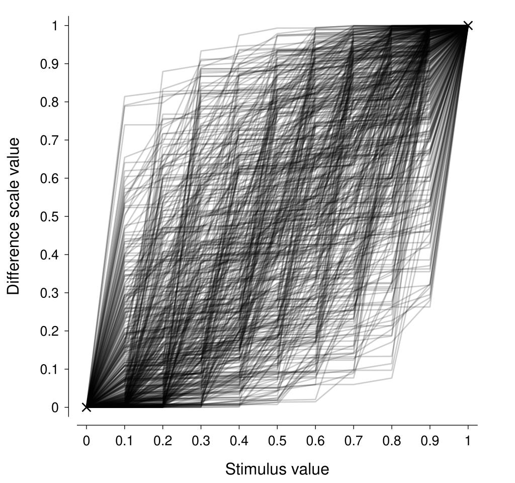
Now, we need to decide on an appropriate value of \(\alpha\). For our purposes, we can interpret this parameter as determining the amount of variability in the change in the difference scale from one stimulus level to the next. A neat way to do that is to visualise repeated draws from the distribution with a particular \(\alpha\) and see how well they represent the sort of difference scales that we would expect to see a-priori. In the figure below, I am showing the difference scales from 500 draws where \(\alpha = 0.3\) and there are 11 stimulus levels (\(K = 11\)). This looks to pretty reasonably encompass the sort of difference scale one might expect to see for a generic stimulus dimension (assuming a positive monotonic difference scale). Increasing values of \(\alpha\) produce difference scales that are more linear.

We also need to think about the parameter describing the variability in the stimulus representation, \(\sigma\). We need our prior to respect the constraint that the standard deviation must be greater than zero, and a half-normal distribution is a common choice for such constraints. To complete the specification of the prior, we need to specify a value for the standard deviation of this half-normal. I find setting \(\sigma\) to half the value at which the parameter becomes highly unlikely to be a useful rule of thumb (Dienes, 2014), so we might set it to something like: $$ \sigma \sim \textrm{half-}\mathcal{N}\left(0.2\right) $$

Example: perceived correlation in scatterplots

Let’s now turn to the previously-mentioned dataset concerning the perception of correlation in scatterplots (Knoblauch & Maloney, 2008) to see how this all works in practice.

Observations

The data reported by Knoblauch & Maloney (2008) consist of three sessions from a single observer, with each session containing 330 trials for a total of 990 trials (\(N = 990\)). We can represent the response data (\(r\)) as a one-dimensional binary array with 990 items, where each item indicates whether the \(\left(x_c, x_d\right)\) pair was considered to be more (coded as 1) or less (coded as 0) perceptually different than the \(\left(x_a, x_b\right)\) pair. We can represent the stimulus information (\(q\)) as a two-dimensional integer array (\(990 \times 4\)), where each row represents a single trial and the four columns represent the indices of the \(x_a, x_b, x_c, x_d\) stimuli. These stimuli were drawn from a set of 11 levels (\(K = 11\)), where \(x = \left(0, 0.1, \dots, 0.9, 0.98\right)\).

Model implementation

Our goal is to implement the Bayesian difference scaling model that has been described above in Python code, using the PyMC library.

As previewed earlier, we first need to specify a way of calculating the normal cumulative distribution function that allows PyMC to do its magic. We can do that by creating a function that uses pm.math.invprobit (rather than our previous use of scipy.stats):

def norm_p_ltz_pm(mu, sigma):
    return pm.math.invprobit(x=(0.0 - mu) / sigma)

Now we can translate the description of the model in the above into PyMC form. Hopefully you will be able to see that there is a fairly direct correspondence between the mathematical description and its PyMC implementation.

def get_model(x, r, q):

    # number of trials
    N = len(r)
    # number of stimulus levels
    K = len(x)

    # check that the quad indices are in the expected format
    assert np.min(q) == 0
    assert q.shape == (N, 4)
    assert (np.max(q) + 1) == K

    n_beta_delta = K - 1

    coords = {
        "beta_delta_num": np.arange(1, n_beta_delta + 1),
        "psi_num": np.arange(1, K + 1),
        "trial_num": np.arange(1, N + 1),
    }

    with pm.Model(coords=coords) as model:

        # stimulus noise
        sigma = pm.HalfNormal("sigma", sigma=0.2)

        # prior on change between successive levels
        concentration = 0.3
        beta_delta = pm.Dirichlet(
            "beta_delta",
            np.ones(n_beta_delta) * concentration,
            dims=("beta_delta_num",),
        )

        beta = beta_delta.cumsum()

        # add lower anchor at 0
        # note that upper anchor is already at 1 in `beta`
        psi = pm.Deterministic(
            "psi",
            pm.math.concatenate(([0.0], beta)),
            dims=("psi_num",),
        )

        # apply the mapping from the stimulus indices to
        # the difference scale
        mu = psi[q]

        # use the psychometric function to obtain the probability
        # of |cd| > |ab|, given (mu, sigma)
        p = pm.Deterministic(
            "p",
            pf(mu=mu, sigma=sigma, norm_p_ltz_func=norm_p_ltz_pm),
            dims=("trial_num",),
        )

        pm.Bernoulli("r", p=p, observed=r, dims=("trial_num",))

    return model

We can then use PyMC’s sample function to produce samples from the posterior distribution.

Model evaluation

After checking that the MCMC diagnostics all seem acceptable, a useful next step (before inspecting the posterior distributions) is to assess whether the fitted model seems to display “descriptive adequacy” (Shiffrin, Lee, Kim, & Wagenmakers, 2008). A particularly informative way to conduct such a check in a Bayesian context is to compare summaries of the raw data against summaries of draws from the fitted model (“posterior predictives”). In doing so, we hope to spot any problematic features of the fitted model.

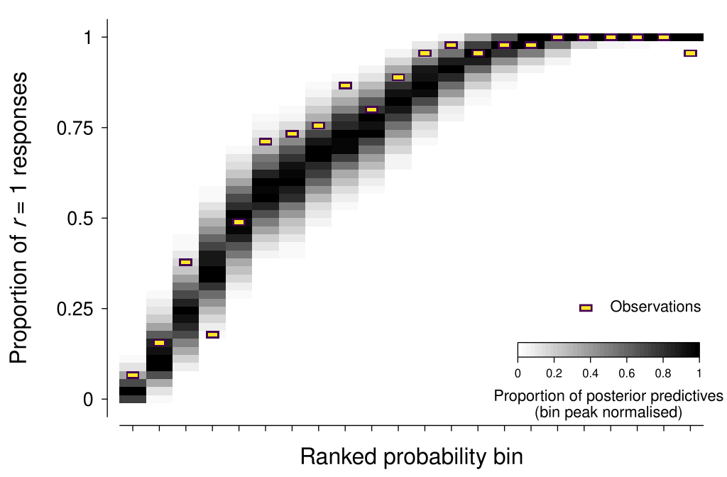
Such posterior predictive checks typically operate informally via visual inspection. However, the data from a difference scaling experiment are challenging to visualise given the four-dimensional variations across trials (the stimulus quadruples). The approach that I have come up with here is to use the sorted median of the posterior distribution for the response probability variable (called p in the model) as a way of grouping trials, and then comparing the observed proportion of \(r = 1\) responses within each bin against the posterior predictives. As shown in the figure below, the model seems to be in reasonable agreement with most of the observation summaries (I will discuss one exception in Additional considerations below).

As Michael Betancourt has mentioned, “posterior retrodictives” is a more accurate term than posterior predictives—given that the same data is used to both fit and evaluate the model. However, I will stick with the better-known form of the term here.

Posterior distributions

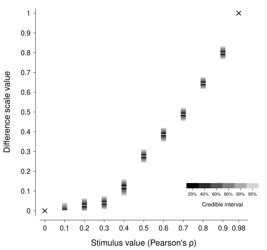
We can now inspect the posterior distribution for the psi parameter in the model to describe the difference scale. As shown in the figure below, the estimated difference scale suggests that scatterplots of the same numerical difference in correlation coefficient have a much smaller perceptual difference for low correlations compared to high correlations. As expected, this scale is similar to that reported by Knoblauch & Maloney (2008)—with differences arising from different representational noise assumptions and our enforcement of positive monotonicity.

To understand the practical consequences of this difference scale, we can compare scatterplots that are equally spaced on the correlation coefficient scale against those that are equally spaced on the estimated perceptual difference scale (a complication here is due to the discreteness of our model of the difference scale; to circumvent this limitation, I have used linear interpolation to produce a continuous difference scale). In the figure below, the scatterplots in the bottom row should appear to have more perceptually-similar changes in apparent correlation compared with those in the top row—if your perception of scatterplot correlations matches that of the observer who generated this data, that is.

Additional considerations

There are a few additional aspects of difference scaling that I have explored in my own forays (Kruse, Mannion, Alenin, & Tyo, 2022; Sun & Mannion, 2021) that may be worth considering (each of which was also mentioned by Knoblauch & Maloney, 2008).

Incorporating the propensity to lapse

Even the most attentive and engaged observer has some non-zero probability of ‘lapsing’ on a given trial—that is, responding independently of the stimuli and task requirements. Lapses can be caused by many factors, such as accidentally pressing the wrong key, blinking at an inopportune time, and momentary mind wandering or distraction. The figure above that shows the posterior predictives for the scatterplot example suggests that there were some lapses evident in that data—note how the observed proportion of \(r = 1\) responses becomes lower than 1 at the far right bin, whereas the model is very confident that we should expect \(r = 1\) responses.

Bayesian models can be readily adapted to accommodate lapsing behaviour (e.g., Martin, 2018, p. 174–175, and Gelman, Hill, & Vehtari, 2020, p. 283). This process can be facilitated by the inclusion of ‘catch’ trials, in which the stimuli are chosen such that any unpredicted responses can be assumed to be only caused by lapses (Prins, 2012). In this context, this could involve trials in which one pair has the smallest possible difference in stimulus levels while the other pair has the largest possible difference.

Extending to multiple observers

We are often interested in characterising the behaviour of a population of observers rather than a single observer (though see the great article by Smith & Little, 2018). To do so in this context, we can extend the model to include “random effects” that allow us to describe both the central tendency and variation across observers. However, as described in the Prior distributions section above, this may require the specification of more accommodating forms of prior distributions or difference scale form assumptions.

Adaptively selecting trial stimuli

The common method of choosing a stimulus quadruple on each trial randomly or pseudo-randomly from the complete set of non-overlapping quadruples is relatively inefficient, with many quadruples not being particularly informative of the difference scale. We have found that using an adaptive approach, such as that described by Kontsevich & Tyler (1999), works very well in reducing the number of trials required for a given level of estimation accuracy.

Acknowledgements

Thanks to Colin Clifford for helpful discussions about the rotation of coordinates method to calculate the probabilities in the psychometric function (any errors are mine).

Software versions

These are the versions of the key software and packages that were used to generate the material in this post:

Python implementation: CPython
Python version       : 3.9.13

numpy    : 1.23.2
veusz    : 3.4
pymc     : 4.1.7
xarray   : 2022.6.0
scipy    : 1.9.1

License

This work is licensed under CC BY-NC-ND 4.0.

References

1. Aguilar, G., Wichmann, F.A., & Maertens, M. (2017) Comparing sensitivity estimates from MLDS and forced-choice methods in a slant-from-texture experiment. Journal of Vision, 17, 1–37.
2. Bürkner, P.-C. & Charpentier, E. (2020) Modelling monotonic effects of ordinal predictors in Bayesian regression models. British Journal of Mathematical and Statistical Psychology, 73(3), 420–451.
3. Charrier, C., Maloney, L.T., Cherifi, H., & Knoblauch, K. (2007) Maximum likelihood difference scaling of image quality in compression-degraded images. Journal of The Optical Society of America A—Optics, Image Science, and Vision, 24(11), 3418–3426.
4. Cheeseman, J.R., Ferwerda, J.A., Maile, F.J., & Fleming, R.W. (2021) Scaling and discriminability of perceived gloss. Journal of The Optical Society of America A—Optics, Image Science, and Vision, 38(2), 203–210.
5. Dienes, Z. (2014) Using Bayes to get the most out of non-significant results. Frontiers in Psychology, 5(781), 1–17.
6. Gelman, A., Vehtari, A., Simpson, D., Margossian, C. C., Carpenter, B., Yao, Y., Kennedy, L., Gabry, J., Bürkner, P.-C., & Modrák, M. (2020) Bayesian workflow. ArXiV, 1–77.
7. Gelman, A., Hill, J., & Vehtari, A. (2020) Regression and other stories. Cambridge University Press.
8. Knoblauch, K. & Maloney, L. (2008) MLDS: Maximum Likelihood Difference Scaling in R. Journal of Statistical Software, 25(2), 1–26.
9. Kontsevich, L.L. & Tyler, C.W. (1999) Bayesian adaptive estimation of psychometric slope and threshold. Vision Research, 39, 2729–2737.
10. Kruse, A.W., Mannion, D.J., Alenin, A., & Tyo, J.S. (2022) User study comparing linearity and orthogonalization for polarimetric visualizations. IEEE Access, 10, 28308–28321.
11. Maloney, L. T. & Yang, J. N. (2003) Maximum likelihood difference scaling. Journal of Vision, 3(8), 573–585.
12. Martin, O. (2018) Bayesian analysis with Python (2nd ed.). Packt Publishing.
13. Prins, N. (2012) The psychometric function: the lapse rate revisited. Journal of Vision, 12(6), 1–16.
14. Shiffrin, R.M., Lee, M.D., Kim, W., & Wagenmakers, E.-J. (2008) A Survey of Model Evaluation Approaches With a Tutorial on Hierarchical Bayesian Methods. Cognitive Science, 32, 1248–1284.
15. Smith, P.L. & Little, D.R. (2018) Small is beautiful: In defense of the small-N design. Psychonomic Bulletin and Review, 25, 2083–2101.
16. Sun, H.-C. & Mannion, D.J. (2021) A comparison of the apparent gloss of rendered objects presented in the lower and upper regions of the visual field. PsyArXiV, 1–14.
17. van de Schoot, R., Depaoli, S., King, R., Kramer, B., Märtens, K., Tadesse, M. G., Vannucci, M., Gelman, A., Veen, D., Willemsen, J., & Yau, C. (2021) Bayesian statistics and modelling. Nature Reviews Methods Primers, 1(1), 1–26.
18. Wagenmakers, E.-J., Marsman, M., Jamil, T., Ly, A., Verhagen, J., Love, J., Selker, R., Gronau, Q. F., Šmíra, M., Epskamp, S., Matzke, D., Rouder, J. N., & Morey, R. D. (2018) Bayesian inference for psychology. Part I: Theoretical advantages and practical ramifications. Psychonomic Bulletin & Review, 25, 35–57.