Spatial frequency filtering
Objectives
- Be able to convert stimuli from image space to frequency space.
- Know how to create spatial frequency filters.
- Be able to apply spatial frequency filters to produce filtered images.
Many groups are interested in using filtering techniques to alter the spatial frequency content of their stimuli. Here, we will learn some of the ways that we can filter images in Python.
Tip
We touch on some advanced concepts in this lesson. You might find it useful to review Data—arrays and numpy to understand our data representations.
Preparing the stimulus
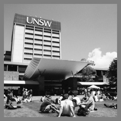
For this lesson, we are going to use the image of UNSW shown below:
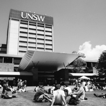
First, however, we need to think about the intensity structure of the image. Because we will be altering such structure during the filtering operations, we want to ensure that we a) preserve important properties of the image, and b) allow sufficient ‘room’ so that we don’t run into floor and ceiling issues (that is, intensities that are outside of the range that we can display).
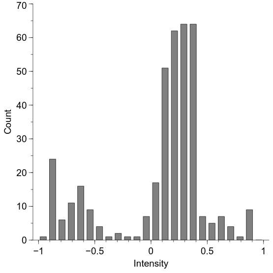
Let’s start by having a look at the intensity histogram of the image. That is, we will count up how many pixels have a particular intensity value for each of a range of intensities between -1 and 1. We get something like below:
We will now adjust the histogram to make it be able to be preserved across our spatial filtering. We will do this by first making the mean intensity to be zero and then alter the standard deviation to be 0.2. This standard deviation is a measure of image contrast, also known as “root mean square” (RMS) contrast. We will see how to do this in code and what effect it has on image appearance below, but here is the effect on the intensity histogram:
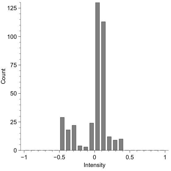
Our aim will be to preserve the mean and standard deviation of this intensity distribution for each of our filtered images.
Displaying altered images in PsychoPy
We have considered previously how to use images from a file on disk (Drawing—images). Here, we wish to do something similar but also slightly different—we want to use an image from a file on disk, but we want to first load it into Python so we can make some alterations to it.
import numpy as np
import scipy.misc

import psychopy.visual
import psychopy.event

win = psychopy.visual.Window(
    size=[400, 400],
    fullscr=False,
    units="pix"
)

# this gives a (y, x) array of values between 0.0 and 255.0
raw_img = scipy.misc.imread(
    "unsw_bw.jpg",
    flatten=True
)

# we first need to convert it to the -1:+1 range
raw_img = (raw_img / 255.0) * 2.0 - 1.0

# we also need to flip it upside-down to match the psychopy convention
raw_img = np.flipud(raw_img)

img = psychopy.visual.ImageStim(
    win=win,
    image=raw_img,
    units="pix",
    size=raw_img.shape
)

img.draw()

win.flip()

psychopy.event.waitKeys()

win.close()
As seen in the above, we first use the function scipy.misc.imread to load the image into the variable raw_img.
After converting it into the -1 to +1 range, we flip it upside-down and then provide ImageStim with the variable raw_img, which contains the direct image data rather than the filename that we have used previously.
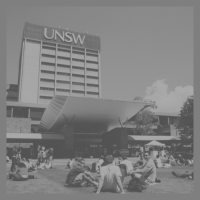
By doing it this way, we can alter the image—such as performing the histogram changes we looked at previously:
import numpy as np
import scipy.misc

import psychopy.visual
import psychopy.event

win = psychopy.visual.Window(
    size=[400, 400],
    fullscr=False,
    units="pix"
)

# this gives a (y, x) array of values between 0.0 and 255.0
raw_img = scipy.misc.imread(
    "unsw_bw.jpg",
    flatten=True
)

# we first need to convert it to the -1:+1 range
raw_img = (raw_img / 255.0) * 2.0 - 1.0

# we also need to flip it upside-down to match the psychopy convention
raw_img = np.flipud(raw_img)

# desired RMS
rms = 0.2

# make the mean to be zero
raw_img = raw_img - np.mean(raw_img)
# make the standard deviation to be 1
raw_img = raw_img / np.std(raw_img)
# make the standard deviation to be the desired RMS
raw_img = raw_img * rms

img = psychopy.visual.ImageStim(
    win=win,
    image=raw_img,
    units="pix",
    size=raw_img.shape
)

img.draw()

win.flip()

psychopy.event.waitKeys()

win.close()
Converting to frequency space
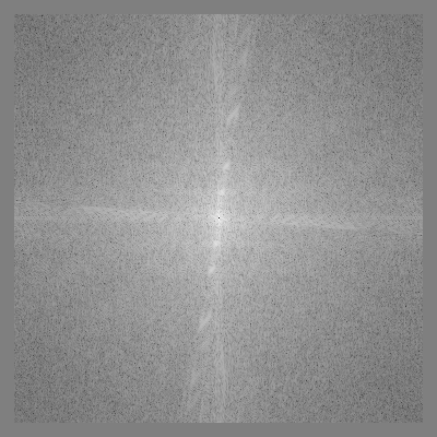
We are going to perform spatial frequency filtering via the frequency domain. That is, we are going to convert our image representation from horizontal and vertical space to a polar representation of orientation (polar angle) and spatial frequency (radius). We are not altering anything about the image in this transformation; we are simply converting it into a more convenient format in which to perform our filtering.
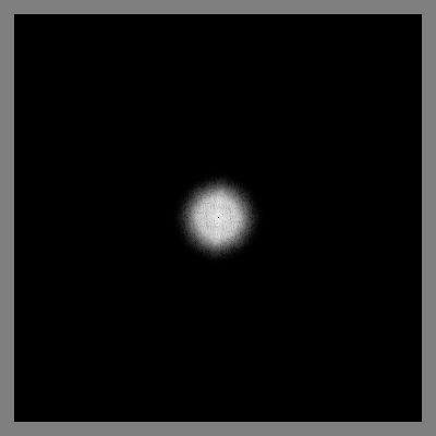
In the below code, we use the fft2 function (Fast Fourier Transform) to convert our image.
We then use the abs function to get the amplitude spectrum, and use fftshift to move the origin to the centre of the image.
Because many of the values are quite small, we use a log transform to make the spectrum easier to see (adding a small value to prevent logs of zero).
import numpy as np
import scipy.misc

import psychopy.visual
import psychopy.event

win = psychopy.visual.Window(
    size=[400, 400],
    fullscr=False,
    units="pix"
)

# this gives a (y, x) array of values between 0.0 and 255.0
raw_img = scipy.misc.imread(
    "unsw_bw.jpg",
    flatten=True
)

# we first need to convert it to the -1:+1 range
raw_img = (raw_img / 255.0) * 2.0 - 1.0

# we also need to flip it upside-down to match the psychopy convention
raw_img = np.flipud(raw_img)

# desired RMS
rms = 0.2

# make the mean to be zero
raw_img = raw_img - np.mean(raw_img)
# make the standard deviation to be 1
raw_img = raw_img / np.std(raw_img)
# make the standard deviation to be the desired RMS
raw_img = raw_img * rms

# convert to frequency domain
img_freq = np.fft.fft2(raw_img)

# calculate amplitude spectrum
img_amp = np.fft.fftshift(np.abs(img_freq))

# for display, take the logarithm
img_amp_disp = np.log(img_amp + 0.0001)

# rescale to -1:+1 for display
img_amp_disp = (
    (
        (img_amp_disp - np.min(img_amp_disp)) * 2
    ) / np.ptp(img_amp_disp)  # 'ptp' = range
) - 1

img = psychopy.visual.ImageStim(
    win=win,
    image=img_amp_disp,
    units="pix",
    size=raw_img.shape
)

img.draw()

win.flip()

win.getMovieFrame()
psychopy.event.waitKeys()

win.close()
What we will do in our spatial frequency filtering is alter the radial structure of this frequency-space representation, and then convert it back into the image domain.
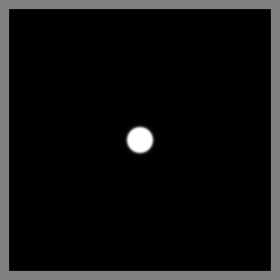
Creating a spatial frequency filter
Here, we will look at how to construct an appropriate spatial frequency filter. We will use the Butterworth class of filters, beginning with a low-pass filter. To create such a filter, we first need to decide on two parameters—the cutoff frequency and the filter ‘order’. The cutoff frequency is typically between 0 and 0.5, and determine the distance from the origin at which the filter response is at half its maximum. The ‘order’ is an integer that determines the steepness of the filter about this value, with higher values giving steeper responses.
We can create a low-pass Butterworth filter in Python using the psychopy.filters.butter2d_lp function.
Let’s see what one looks like:
import numpy as np
import scipy.misc

import psychopy.visual
import psychopy.event
import psychopy.filters

win = psychopy.visual.Window(
    size=[400, 400],
    fullscr=False,
    units="pix"
)

# this gives a (y, x) array of values between 0.0 and 255.0
raw_img = scipy.misc.imread(
    "unsw_bw.jpg",
    flatten=True
)

# we first need to convert it to the -1:+1 range
raw_img = (raw_img / 255.0) * 2.0 - 1.0

# we also need to flip it upside-down to match the psychopy convention
raw_img = np.flipud(raw_img)

# desired RMS
rms = 0.2

# make the mean to be zero
raw_img = raw_img - np.mean(raw_img)
# make the standard deviation to be 1
raw_img = raw_img / np.std(raw_img)
# make the standard deviation to be the desired RMS
raw_img = raw_img * rms

# convert to frequency domain
img_freq = np.fft.fft2(raw_img)

# calculate amplitude spectrum
img_amp = np.fft.fftshift(np.abs(img_freq))

lp_filt = psychopy.filters.butter2d_lp(
    size=raw_img.shape,
    cutoff=0.05,
    n=10
)

# 'lp_filt' will be 0:1; convert it to -1:1 for display
lp_filt_disp = lp_filt * 2.0 - 1.0

img = psychopy.visual.ImageStim(
    win=win,
    image=lp_filt_disp,
    units="pix",
    size=raw_img.shape
)

img.draw()

win.flip()

psychopy.event.waitKeys()

win.close()
Applying a spatial frequency filter
To apply our filter, we simply multiply the frequency-space representation of our image by the filter shown above:
import numpy as np
import scipy.misc

import psychopy.visual
import psychopy.event
import psychopy.filters

win = psychopy.visual.Window(
    size=[400, 400],
    fullscr=False,
    units="pix"
)

# this gives a (y, x) array of values between 0.0 and 255.0
raw_img = scipy.misc.imread(
    "unsw_bw.jpg",
    flatten=True
)

# we first need to convert it to the -1:+1 range
raw_img = (raw_img / 255.0) * 2.0 - 1.0

# we also need to flip it upside-down to match the psychopy convention
raw_img = np.flipud(raw_img)

# desired RMS
rms = 0.2

# make the mean to be zero
raw_img = raw_img - np.mean(raw_img)
# make the standard deviation to be 1
raw_img = raw_img / np.std(raw_img)
# make the standard deviation to be the desired RMS
raw_img = raw_img * rms

# convert to frequency domain
img_freq = np.fft.fft2(raw_img)

# calculate amplitude spectrum
img_amp = np.fft.fftshift(np.abs(img_freq))

lp_filt = psychopy.filters.butter2d_lp(
    size=raw_img.shape,
    cutoff=0.05,
    n=10
)

img_filt = np.fft.fftshift(img_freq) * lp_filt

img_filt_amp = np.abs(img_filt)

# for display, take the logarithm
img_filt_amp_disp = np.log(img_filt_amp + 0.0001)

# rescale to -1:+1 for display
img_filt_amp_disp = (
    (
        (img_filt_amp_disp - np.min(img_filt_amp_disp)) * 2
    ) / np.ptp(img_filt_amp_disp)  # 'ptp' = range
) - 1

img = psychopy.visual.ImageStim(
    win=win,
    image=img_filt_amp_disp,
    units="pix",
    size=raw_img.shape
)

img.draw()

win.flip()

psychopy.event.waitKeys()

win.close()
Converting back to an image
Now that we have our altered frequency-space representation, we convert it back to image-space by performing the inverse of the operations we performed to get it into frequency-space.
import numpy as np
import scipy.misc

import psychopy.visual
import psychopy.event
import psychopy.filters

win = psychopy.visual.Window(
    size=[400, 400],
    fullscr=False,
    units="pix"
)

# this gives a (y, x) array of values between 0.0 and 255.0
raw_img = scipy.misc.imread(
    "unsw_bw.jpg",
    flatten=True
)

# we first need to convert it to the -1:+1 range
raw_img = (raw_img / 255.0) * 2.0 - 1.0

# we also need to flip it upside-down to match the psychopy convention
raw_img = np.flipud(raw_img)

# desired RMS
rms = 0.2

# make the mean to be zero
raw_img = raw_img - np.mean(raw_img)
# make the standard deviation to be 1
raw_img = raw_img / np.std(raw_img)
# make the standard deviation to be the desired RMS
raw_img = raw_img * rms

# convert to frequency domain
img_freq = np.fft.fft2(raw_img)

# calculate amplitude spectrum
img_amp = np.fft.fftshift(np.abs(img_freq))

lp_filt = psychopy.filters.butter2d_lp(
    size=raw_img.shape,
    cutoff=0.05,
    n=10
)

img_filt = np.fft.fftshift(img_freq) * lp_filt

# convert back to an image
img_new = np.real(np.fft.ifft2(np.fft.ifftshift(img_filt)))

# convert to mean zero and specified RMS contrast
img_new = img_new - np.mean(img_new)
img_new = img_new / np.std(img_new)
img_new = img_new * rms

# there may be some stray values outside of the presentable range; convert < -1
# to -1 and > 1 to 1
img_new = np.clip(img_new, a_min=-1.0, a_max=1.0)

img = psychopy.visual.ImageStim(
    win=win,
    image=img_new,
    units="pix",
    size=raw_img.shape
)

img.draw()

win.flip()

psychopy.event.waitKeys()

win.close()
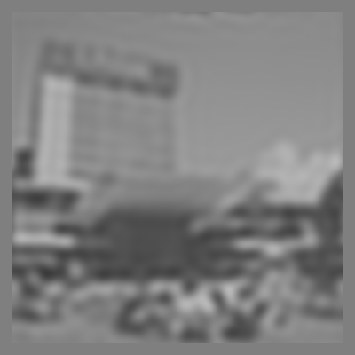
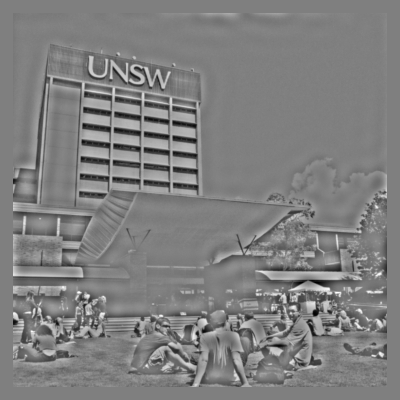
And we have our low-pass filtered image!
Other spatial frequency filters
The above process was for a low-pass filter, but similar strategies can be adopted for high-pass and band-pass filters.
For a high-pass filter, you can use psychopy.filters.butter2d_hp, which has similar arguments as the low-pass filter.
For a band-pass filter, you can use psychopy.filters.butted2d_bp, which requires separate cutoff frequencies for the inner and outer frequencies that define the inclusive frequency band.
Here is an example of a high-pass filter in action:
import numpy as np
import scipy.misc

import psychopy.visual
import psychopy.event
import psychopy.filters

win = psychopy.visual.Window(
    size=[400, 400],
    fullscr=False,
    units="pix"
)

# this gives a (y, x) array of values between 0.0 and 255.0
raw_img = scipy.misc.imread(
    "unsw_bw.jpg",
    flatten=True
)

# we first need to convert it to the -1:+1 range
raw_img = (raw_img / 255.0) * 2.0 - 1.0

# we also need to flip it upside-down to match the psychopy convention
raw_img = np.flipud(raw_img)

# desired RMS
rms = 0.2

# make the mean to be zero
raw_img = raw_img - np.mean(raw_img)
# make the standard deviation to be 1
raw_img = raw_img / np.std(raw_img)
# make the standard deviation to be the desired RMS
raw_img = raw_img * rms

# convert to frequency domain
img_freq = np.fft.fft2(raw_img)

# calculate amplitude spectrum
img_amp = np.fft.fftshift(np.abs(img_freq))

hp_filt = psychopy.filters.butter2d_hp(
    size=raw_img.shape,
    cutoff=0.05,
    n=10
)

img_filt = np.fft.fftshift(img_freq) * hp_filt

# convert back to an image
img_new = np.real(np.fft.ifft2(np.fft.ifftshift(img_filt)))

# convert to mean zero and specified RMS contrast
img_new = img_new - np.mean(img_new)
img_new = img_new / np.std(img_new)
img_new = img_new * rms

# there may be some stray values outside of the presentable range; convert < -1
# to -1 and > 1 to 1
img_new = np.clip(img_new, a_min=-1.0, a_max=1.0)

img = psychopy.visual.ImageStim(
    win=win,
    image=img_new,
    units="pix",
    size=raw_img.shape
)

img.draw()

win.flip()

psychopy.event.waitKeys()

win.close()