Descriptive statistics—calculation and visualisation

In this lesson, we will be investigating how we can use Python to calculate basic (but important) descriptive statistics—including bootstrapping approaches that leverage the power of programming. We will also be learning more about figure creation, including how to accommodate the common requirement for a figure to have multiple panels and about two new figure types (boxplots and error plots).

Warning

This is a long lesson and covers a fair bit of ground.

Generating some data

Typically, the process would begin with the loading of data produced from an experiment. Here, to simplify things, we will instead simulate the data that might have been produced by an experiment. In particular, we will simulate the outcome of a between-subjects experiment with 3 conditions/groups and 30 participants per group. In our data, the three conditions are represented by normal distributions with different means and standard deviations. To make the subsequent code examples more concise, we will save the generated data to a text file that we can then load as required.

import numpy as np

# how many (simulated) participants in each group
n_per_group = 30

# mean of each group's distribution
group_means = [1.0, 2.0, 3.0]
# set the standard deviation of each group to be half of its mean
group_stdevs = [0.5, 1.0, 1.5]

n_groups = len(group_means)

# create an empty array where rows are participants and columns are groups
data = np.empty([n_per_group, n_groups])
# fill it with a special data type, 'nan' (Not A Number)
data.fill(np.nan)

for i_group in range(n_groups):

    group_mean = group_means[i_group]
    group_stdev = group_stdevs[i_group]

    # generate the group data by sampling from a normal distribution with the
    # group's parameters
    group_data = np.random.normal(
        loc=group_mean,
        scale=group_stdev,
        size=n_per_group
    )

    data[:, i_group] = group_data

# check that we have generated all the data we expected to
assert np.sum(np.isnan(data)) == 0

# let's have a look at the first five 'participants'
print data[:5, :]

# and save
data_path = "prog_data_vis_descriptives_sim_data.tsv"

np.savetxt(
    data_path,
    data,
    delimiter="\t",
    header="Simulated data for the Descriptives lesson"
)

[[ 1.30850199  1.4439598   6.56498381]
 [ 0.96473397  1.12874056  1.20549073]
 [ 1.08706521  1.57177425  4.8045448 ]
 [ 0.4133616   1.53001941  3.90450457]
 [-0.06627179  0.47766485  1.90061235]]

Most of the above code will be familiar, with the exception of a new statement—assert. The assert statement is quite simple: if the following boolean does not evaluate to True, then Python raises an error. Here, we are using it to verify that we have filled up our array like we expected to. The function np.isnan returns a boolean array with elements having the value of True where the corresponding element in the input array is nan, and False otherwise. Then, we use np.sum to count up all the True values. If we have filled up our data array correctly, then there won’t be any nan elements so the sum will be zero and we can happily proceed with the rest of the code. But if there are nan values in there, we’ve made a mistake and the program will notify us. The assert statement is a very useful way of verifying that aspects of the code are doing what you think, and it is often good practice to include assert statements quite liberally.

Visualising the distributions

The first thing we will do is take a look at the distributions using the histogram technique we encountered in the previous lesson. However, we have three conditions here—we could think about including them all in the one histogram, but it might get a bit crowded. Instead, we will create a figure with multiple panels, each showing the histogram for one condition.

One of the primary purposes of generating such a figure is to be able to compare the distributions across the three conditions. Hence, a vertical stacking of panels would seem to be better than horizontal stacking because it would allow a direct comparison of density by looking down the page. So let’s generate a one-column figure (8.4cm wide) with three vertical panels (16cm high).

First, we will setup up the framework for our figure like we have done previously:

import numpy as np

import veusz.embed

data_path = "prog_data_vis_descriptives_sim_data.tsv"

# load the data we generated in the previous step
data = np.loadtxt(data_path, delimiter="\t")

# pull out some design parameters from the shape of the array
n_per_group = data.shape[0]
n_cond = data.shape[1]

embed = veusz.embed.Embedded("veusz")

page = embed.Root.Add("page")
page.width.val = "8.4cm"
page.height.val = "16cm"

embed.WaitForClose()

Previously, we added a graph element directly to the page. Here, we want to have multiple panels so we first add a grid element to the page. Such a grid has two particularly important properties, rows and columns. Here, we want just the one column and three rows (to have our three panels stacked vertically).

import numpy as np

import veusz.embed

data_path = "prog_data_vis_descriptives_sim_data.tsv"

# load the data we generated in the previous step
data = np.loadtxt(data_path, delimiter="\t")

# pull out some design parameters from the shape of the array
n_per_group = data.shape[0]
n_cond = data.shape[1]

embed = veusz.embed.Embedded("veusz")

page = embed.Root.Add("page")
page.width.val = "8.4cm"
page.height.val = "16cm"

grid = page.Add("grid")

grid.rows.val = int(n_cond)
grid.columns.val = 1

embed.WaitForClose()

Now, rather than adding the graph to the page, we add it to the grid. Consecutive graphs will then appear in different panels:

import numpy as np

import veusz.embed

data_path = "prog_data_vis_descriptives_sim_data.tsv"

# load the data we generated in the previous step
data = np.loadtxt(data_path, delimiter="\t")

# pull out some design parameters from the shape of the array
n_per_group = data.shape[0]
n_cond = data.shape[1]

embed = veusz.embed.Embedded("veusz")

page = embed.Root.Add("page")
page.width.val = "8.4cm"
page.height.val = "16cm"

grid = page.Add("grid")

grid.rows.val = int(n_cond)
grid.columns.val = 1

for i_cond in range(n_cond):

    graph = grid.Add("graph", autoadd=False)

    x_axis = graph.Add("axis")
    y_axis = graph.Add("axis")

embed.WaitForClose()

Ok, now we are getting somewhere! We have the basic framework for our three panels, now we need to ‘fill’ each panel.

We are going to be making histograms, and the first important decision we need to make are the positions of the ‘bins’. Because we want to compare across the three panels, it is desirable for them to all have the same bins. One plausible way of deciding the bins is to use the minimum and maximum values across all conditions as the bin extremes. We’ll add a small amount of padding as well to give them a bit of room at the edges. Then, we will use the np.linspace to generate a series of values between the extremes. Then, because we have defined the bin edges but we want to plot the bin centres, we work out the bin size (as the difference between two adjacent edges) and add half that size to each edge. Finally, we make veusz aware of our bin centres, which will apply to each of the figure panels. Because the last bin edge doesn’t contribute to the counts, we don’t include the last bin.

import numpy as np

import veusz.embed

data_path = "prog_data_vis_descriptives_sim_data.tsv"

# load the data we generated in the previous step
data = np.loadtxt(data_path, delimiter="\t")

# pull out some design parameters from the shape of the array
n_per_group = data.shape[0]
n_cond = data.shape[1]

embed = veusz.embed.Embedded("veusz")

page = embed.Root.Add("page")
page.width.val = "8.4cm"
page.height.val = "16cm"

grid = page.Add("grid")

grid.rows.val = int(n_cond)
grid.columns.val = 1

min_val = np.min(data)
max_val = np.max(data)

bin_pad = 0.5

n_bins = 20

bin_edges = np.linspace(
    min_val - bin_pad,
    max_val + bin_pad,
    n_bins,
    endpoint=True
)

bin_delta = bin_edges[1] - bin_edges[0]

bin_centres = bin_edges + (bin_delta / 2.0)

embed.SetData("bin_centres", bin_centres[:-1])

for i_cond in range(n_cond):

    graph = grid.Add("graph", autoadd=False)

    x_axis = graph.Add("axis")
    y_axis = graph.Add("axis")

embed.WaitForClose()

Now, we can calculate the histogram for each condition and use the same techniques that we used previously to plot the histograms as bar graphs. We will also set some properties of the plots to improve their appearance, like we have done previously.

import numpy as np

import veusz.embed

data_path = "prog_data_vis_descriptives_sim_data.tsv"

# load the data we generated in the previous step
data = np.loadtxt(data_path, delimiter="\t")

# pull out some design parameters from the shape of the array
n_per_group = data.shape[0]
n_cond = data.shape[1]

embed = veusz.embed.Embedded("veusz")

page = embed.Root.Add("page")
page.width.val = "8.4cm"
page.height.val = "16cm"

grid = page.Add("grid")

grid.rows.val = int(n_cond)
grid.columns.val = 1

min_val = np.min(data)
max_val = np.max(data)

bin_pad = 0.5

n_bins = 20

bin_edges = np.linspace(
    min_val - bin_pad,
    max_val + bin_pad,
    n_bins,
    endpoint=True
)

bin_delta = bin_edges[1] - bin_edges[0]

bin_centres = bin_edges + (bin_delta / 2.0)

embed.SetData("bin_centres", bin_centres[:-1])

for i_cond in range(n_cond):

    graph = grid.Add("graph", autoadd=False)

    x_axis = graph.Add("axis")
    y_axis = graph.Add("axis")

    hist_result = np.histogram(data[:, i_cond], bin_edges)

    bin_counts = hist_result[0]

    bin_counts_str = "bin_counts_{i:d}".format(i=i_cond)

    embed.SetData(bin_counts_str, bin_counts)

    bar = graph.Add("bar")

    bar.posn.val = "bin_centres"
    bar.lengths.val = bin_counts_str

    graph.Border.hide.val = True

    typeface = "Arial"

    for curr_axis in [x_axis, y_axis]:

        curr_axis.Label.font.val = typeface
        curr_axis.TickLabels.font.val = typeface

        curr_axis.autoMirror.val = False
        curr_axis.outerticks.val = True

embed.WaitForClose()

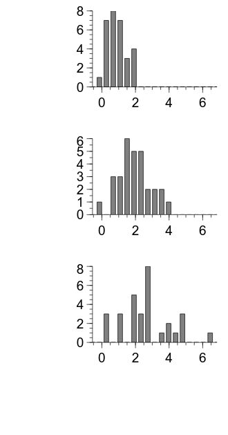
Something that is apparent in the above output is that the left and bottom margins are unnecessarily large. We can change the margins using the leftMargin and bottomMargin properties of the grid:

import numpy as np

import veusz.embed

data_path = "prog_data_vis_descriptives_sim_data.tsv"

# load the data we generated in the previous step
data = np.loadtxt(data_path, delimiter="\t")

# pull out some design parameters from the shape of the array
n_per_group = data.shape[0]
n_cond = data.shape[1]

embed = veusz.embed.Embedded("veusz")

page = embed.Root.Add("page")
page.width.val = "8.4cm"
page.height.val = "16cm"

grid = page.Add("grid")

grid.rows.val = int(n_cond)
grid.columns.val = 1

grid.leftMargin.val = "0.5cm"
grid.bottomMargin.val = "0.5cm"

min_val = np.min(data)
max_val = np.max(data)

bin_pad = 0.5

n_bins = 20

bin_edges = np.linspace(
    min_val - bin_pad,
    max_val + bin_pad,
    n_bins,
    endpoint=True
)

bin_delta = bin_edges[1] - bin_edges[0]

bin_centres = bin_edges + (bin_delta / 2.0)

embed.SetData("bin_centres", bin_centres[:-1])

for i_cond in range(n_cond):

    graph = grid.Add("graph", autoadd=False)

    x_axis = graph.Add("axis")
    y_axis = graph.Add("axis")

    hist_result = np.histogram(data[:, i_cond], bin_edges)

    bin_counts = hist_result[0]

    bin_counts_str = "bin_counts_{i:d}".format(i=i_cond)

    embed.SetData(bin_counts_str, bin_counts)

    bar = graph.Add("bar")

    bar.posn.val = "bin_centres"
    bar.lengths.val = bin_counts_str

    graph.Border.hide.val = True

    typeface = "Arial"

    for curr_axis in [x_axis, y_axis]:

        curr_axis.Label.font.val = typeface
        curr_axis.TickLabels.font.val = typeface

        curr_axis.autoMirror.val = False
        curr_axis.outerticks.val = True

embed.WaitForClose()

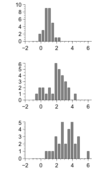
There are a couple of things that need improving about the figure, but it is looking pretty good.

Calculating descriptive statistics

We have visualised our data distributions, and now we can look at how we can calculate descriptive statistics that capture particular aspects of such distributions. Such descriptive statistics are straightforward in Python. The key aspect of our usage of the relevant functions is to specify the axis=0 keyword; this tells Python to perform the relevant operation over the first axis, which is ‘participants’ in our array structure.

import numpy as np

data_path = "prog_data_vis_descriptives_sim_data.tsv"

# load the data we generated in the previous step
data = np.loadtxt(data_path, delimiter="\t")

# central tendency
print "Mean:", np.mean(data, axis=0)
print "Median:", np.median(data, axis=0)

# dispersion
print "Standard deviation:", np.std(data, axis=0, ddof=1)
print "Range:", np.ptp(data, axis=0)

Mean: [ 0.85436068  1.92455729  2.62189693]
Median: [ 0.77348968  1.79358265  2.58372474]
Standard deviation: [ 0.54662476  0.99939682  1.443633  ]
Range: [ 1.93363292  4.43164302  6.19582459]

We generated our data from known distributions, and we can see the means and standard deviations follow our specifications pretty closely.

The names of the numpy functions are mostly intuitive with their functionality (with the exception of ptp for range; ptp is ‘peak-to-peak’). One potentially mysterious argument is ddof=1 for the standard deviation. If we look at the help for np.std, we can see that this corresponds to the value that N is reduced by in the denominator of the standard deviation calculation. With the default value of 0, this corresponds to the population standard deviation. Because we want the sample standard deviation, setting ddof=1 corresponds to using N - 1 in the denominator.

Visualising the distributions via boxplots

Boxplots are a very useful way of visualising distributions. We can create a boxplot in veusz by following the techniques we have used previously to create a graph, and then adding a boxplot element to the graph. We set the values property of the boxplot for each condition to the data array for that condition, and veusz calculates the relevant descriptive statistics and creates the boxplot. We also use the posn property to position each boxplot along the x axis corresponding to that condition’s index.

import numpy as np

import veusz.embed

data_path = "prog_data_vis_descriptives_sim_data.tsv"

# load the data we generated in the previous step
data = np.loadtxt(data_path, delimiter="\t")

# pull out some design parameters from the shape of the array
n_per_group = data.shape[0]
n_cond = data.shape[1]

embed = veusz.embed.Embedded("veusz")

page = embed.Root.Add("page")
page.width.val = "8.4cm"
page.height.val = "10cm"

graph = page.Add("graph", autoadd=False)

x_axis = graph.Add("axis")
y_axis = graph.Add("axis")

for i_cond in range(n_cond):

    box_str = "box_data_{i:d}".format(i=i_cond)

    embed.SetData(box_str, data[:, i_cond])

    boxplot = graph.Add("boxplot")

    boxplot.values.val = box_str
    boxplot.posn.val = i_cond

embed.WaitForClose()

embed.Export("d4a.png", backcolor="white")

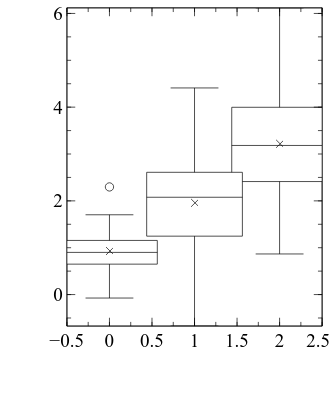
In each boxplot, the horizontal line is the median, the cross is the mean, the top and bottom of the ‘boxes’ are the 75th and 25th percentile, and the ‘whiskers’ extend 1.5 times the inter-quartile range beyond the 25th and 75th percentiles. Any values that lie outside the whiskers are marked individually as circles.

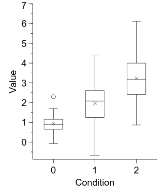
The current plot looks a bit ugly, though—let’s spruce it up a bit. We will first use techniques that are mostly familiar by now.

import numpy as np

import veusz.embed

data_path = "prog_data_vis_descriptives_sim_data.tsv"

# load the data we generated in the previous step
data = np.loadtxt(data_path, delimiter="\t")

# pull out some design parameters from the shape of the array
n_per_group = data.shape[0]
n_cond = data.shape[1]

embed = veusz.embed.Embedded("veusz")

page = embed.Root.Add("page")
page.width.val = "8.4cm"
page.height.val = "10cm"

graph = page.Add("graph", autoadd=False)

x_axis = graph.Add("axis")
y_axis = graph.Add("axis")

for i_cond in range(n_cond):

    box_str = "box_data_{i:d}".format(i=i_cond)

    embed.SetData(box_str, data[:, i_cond])

    boxplot = graph.Add("boxplot")

    boxplot.values.val = box_str
    boxplot.posn.val = i_cond

    # reduce the 'width' of each box
    boxplot.fillfraction.val = 0.3

x_axis.MajorTicks.manualTicks.val = range(n_cond)
x_axis.MinorTicks.hide.val = True
x_axis.label.val = "Condition"

y_axis.min.val = float(np.min(data) - 0.2)
y_axis.label.val = "Value"

# do the typical manipulations to the axis apperances
graph.Border.hide.val = True

typeface = "Arial"

for curr_axis in [x_axis, y_axis]:

    curr_axis.Label.font.val = typeface
    curr_axis.TickLabels.font.val = typeface

    curr_axis.autoMirror.val = False
    curr_axis.outerticks.val = True

embed.WaitForClose()

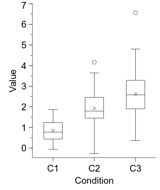
It is looking a lot better now, but one anomaly is that the x axis specifies numerical position values whereas they are really categorical condition labels. We can use strings instead of numbers in veusz by associating each boxplot with a label and telling the x axis to use such labels on the ‘ticks’:

import numpy as np

import veusz.embed

data_path = "prog_data_vis_descriptives_sim_data.tsv"

# load the data we generated in the previous step
data = np.loadtxt(data_path, delimiter="\t")

# pull out some design parameters from the shape of the array
n_per_group = data.shape[0]
n_cond = data.shape[1]

embed = veusz.embed.Embedded("veusz")

page = embed.Root.Add("page")
page.width.val = "8.4cm"
page.height.val = "10cm"

graph = page.Add("graph", autoadd=False)

x_axis = graph.Add("axis")
y_axis = graph.Add("axis")

cond_labels = ["C1", "C2", "C3"]

for i_cond in range(n_cond):

    box_str = "box_data_{i:d}".format(i=i_cond)

    embed.SetData(box_str, data[:, i_cond])

    boxplot = graph.Add("boxplot")

    boxplot.values.val = box_str
    boxplot.posn.val = i_cond
    boxplot.labels.val = cond_labels[i_cond]

    # reduce the 'width' of each box
    boxplot.fillfraction.val = 0.3

x_axis.mode.val = "labels"
x_axis.MajorTicks.manualTicks.val = range(n_cond)
x_axis.MinorTicks.hide.val = True
x_axis.label.val = "Condition"

y_axis.min.val = float(np.min(data) - 0.2)
y_axis.label.val = "Value"

# do the typical manipulations to the axis apperances
graph.Border.hide.val = True

typeface = "Arial"

for curr_axis in [x_axis, y_axis]:

    curr_axis.Label.font.val = typeface
    curr_axis.TickLabels.font.val = typeface

    curr_axis.autoMirror.val = False
    curr_axis.outerticks.val = True

embed.WaitForClose()

Computing confidence intervals

We are often interested in the means of our distributions. The typical way to calculate 95% confidence intervals (CIs) is via the standard error of the mean:

import numpy as np

data_path = "prog_data_vis_descriptives_sim_data.tsv"

# load the data we generated in the previous step
data = np.loadtxt(data_path, delimiter="\t")

# pull out some design parameters from the shape of the array
n_per_group = data.shape[0]
n_cond = data.shape[1]

# calculate standard error of each condition as the sample standard deviation
# divided by sqrt n
sem = np.std(data, axis=0, ddof=1) / np.sqrt(n_per_group)

print "SEMs: ", sem

for i_cond in xrange(n_cond):

    cond_mean = np.mean(data[:, i_cond])
    cond_sem = sem[i_cond]

    lower_ci = cond_mean - 1.96 * cond_sem
    upper_ci = cond_mean + 1.96 * cond_sem

    print "{i:d}: M = {m:.3f}, 95% CI [{lci:.3f}, {uci:.3f}]".format(
        i=i_cond + 1,
        m=cond_mean,
        lci=lower_ci,
        uci=upper_ci
    )

SEMs:  [ 0.09979957  0.18246406  0.26357012]
1: M = 0.854, 95% CI [0.659, 1.050]
2: M = 1.925, 95% CI [1.567, 2.282]
3: M = 2.622, 95% CI [2.105, 3.138]

Here, we will use an alternative non-parametric method called bootstrapping to calculate the CIs. This is a flexible technique that can be usefully applied to many data analysis situations. It is particularly interesting for our purposes because it requires a substantial amount of computation—yet is straightforward to implement once you know the fundamentals of programming.

The key to bootstrapping is to perform resampling with replacement. For example, generating the 95% CI for the mean of a given condition would involve randomly sample a group of participants with replacement—that is, a given participant could appear in the sampled data multiple times, or not at all. Let’s first take a look at how we can do this:

import numpy as np

# generate subject indices from 0 to 9
subjects = range(10)

rand_subj_sample = np.random.choice(
    a=subjects,
    replace=True,
    size=10
)

print rand_subj_sample

[5 9 3 4 8 9 9 2 9 6]

As you can see in the above, we are randomly choosing with replacement a subset of the available participants. Once we have them, we can then pull out their data and compute a mean. Let’s see it in action in the context of the first condition of the data we have been looking at:

import numpy as np

data_path = "prog_data_vis_descriptives_sim_data.tsv"

# load the data we generated in the previous step
data = np.loadtxt(data_path, delimiter="\t")

# pull out some design parameters from the shape of the array
n_per_group = data.shape[0]
n_cond = data.shape[1]

subjects = range(n_per_group)

rand_subj_sample = np.random.choice(
    a=subjects,
    replace=True,
    size=n_per_group
)

boot_data = np.mean(data[rand_subj_sample, 0])

print boot_data

0.993642677268

Bootstrapping involves performing this procedure many, many times. We will use 10,000 iterations here to establish our bootstrapped distribution. When we have calculated such a large number of such means, we can rank the values and look at the 2.5% and 97.5% values as our 95% confidence intervals. The function scipy.stats.scoreatpercentile is very handy for such a calculation:

import numpy as np

import scipy.stats

data_path = "prog_data_vis_descriptives_sim_data.tsv"

# load the data we generated in the previous step
data = np.loadtxt(data_path, delimiter="\t")

# pull out some design parameters from the shape of the array
n_per_group = data.shape[0]
n_cond = data.shape[1]

subjects = range(n_per_group)

n_boot = 10000

boot_data = np.empty(n_boot)
boot_data.fill(np.nan)

for i_boot in range(n_boot):

    rand_subj_sample = np.random.choice(
        a=subjects,
        replace=True,
        size=n_per_group
    )

    boot_data[i_boot] = np.mean(data[rand_subj_sample, 0])

cond_mean = np.mean(boot_data)
lower_ci = scipy.stats.scoreatpercentile(boot_data, 2.5)
upper_ci = scipy.stats.scoreatpercentile(boot_data, 97.5)

print "{i:d}: M = {m:.3f}, 95% CI [{lci:.3f}, {uci:.3f}]".format(
    i=1,
    m=cond_mean,
    lci=lower_ci,
    uci=upper_ci
)

1: M = 0.932, 95% CI [0.749, 1.119]

As you can see, it produces similar results to our previous method using the parametric approach.

Visualising condition means via error plots

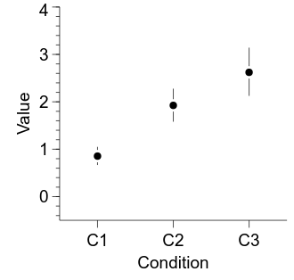
Often a key figure when reporting research is a comparison of means across conditions, almost always with an indication of the uncertainty (‘error’) associated with each mean estimate. Here, we will plot the means and bootstrapped 95% CIs for each of our conditions. We will depict each mean as a point, with bars indicating the 95% CIs.

We begin by setting up our figure framework, as usual:

import numpy as np

import veusz.embed

data_path = "prog_data_vis_descriptives_sim_data.tsv"

# load the data we generated in the previous step
data = np.loadtxt(data_path, delimiter="\t")

# pull out some design parameters from the shape of the array
n_per_group = data.shape[0]
n_cond = data.shape[1]

embed = veusz.embed.Embedded("veusz")

page = embed.Root.Add("page")
page.width.val = "8.4cm"
page.height.val = "8cm"

graph = page.Add("graph", autoadd=False)

x_axis = graph.Add("axis")
y_axis = graph.Add("axis")

embed.WaitForClose()

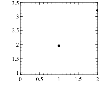
Now, we are going to use a new graph type, xy, to plot our means:

import numpy as np

import veusz.embed

data_path = "prog_data_vis_descriptives_sim_data.tsv"

# load the data we generated in the previous step
data = np.loadtxt(data_path, delimiter="\t")

# pull out some design parameters from the shape of the array
n_per_group = data.shape[0]
n_cond = data.shape[1]

embed = veusz.embed.Embedded("veusz")

page = embed.Root.Add("page")
page.width.val = "8.4cm"
page.height.val = "8cm"

graph = page.Add("graph", autoadd=False)

x_axis = graph.Add("axis")
y_axis = graph.Add("axis")

for i_cond in range(n_cond):

    cond_mean = np.mean(data[:, i_cond])

    data_str = "cond_{i:d}".format(i=i_cond)

    # cond_mean is a single value whereas SetData is expecting a list or array,
    # so pass a one-item list
    embed.SetData(data_str, [cond_mean])

    xy = graph.Add("xy")

    xy.xData.val = i_cond
    xy.yData.val = data_str

embed.WaitForClose()

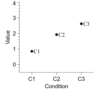
Let’s clean up the figure now, before we add in the CIs:

import numpy as np

import veusz.embed

data_path = "prog_data_vis_descriptives_sim_data.tsv"

# load the data we generated in the previous step
data = np.loadtxt(data_path, delimiter="\t")

# pull out some design parameters from the shape of the array
n_per_group = data.shape[0]
n_cond = data.shape[1]

embed = veusz.embed.Embedded("veusz")

page = embed.Root.Add("page")
page.width.val = "8.4cm"
page.height.val = "8cm"

graph = page.Add("graph", autoadd=False)

x_axis = graph.Add("axis")
y_axis = graph.Add("axis")

cond_labels = ["C1", "C2", "C3"]

for i_cond in range(n_cond):

    cond_mean = np.mean(data[:, i_cond])

    data_str = "cond_{i:d}".format(i=i_cond)

    # cond_mean is a single value whereas SetData is expecting a list or array,
    # so pass a one-item list
    embed.SetData(data_str, [cond_mean])

    xy = graph.Add("xy")

    xy.xData.val = i_cond
    xy.yData.val = data_str
    xy.labels.val = cond_labels[i_cond]

x_axis.mode.val = "labels"
x_axis.MajorTicks.manualTicks.val = range(n_cond)
x_axis.MinorTicks.hide.val = True
x_axis.label.val = "Condition"
x_axis.min.val = -0.5
x_axis.max.val = 2.5

y_axis.min.val = -0.5
y_axis.max.val = 4.0
y_axis.label.val = "Value"

# do the typical manipulations to the axis apperances
graph.Border.hide.val = True

typeface = "Arial"

for curr_axis in [x_axis, y_axis]:

    curr_axis.Label.font.val = typeface
    curr_axis.TickLabels.font.val = typeface

    curr_axis.autoMirror.val = False
    curr_axis.outerticks.val = True

embed.WaitForClose()

OK, now we can compute our 95% CIs and add them in to the figure. We do this by using an extra set of arguments to the SetData function: poserr (positive error) and negerr (negative error). These determine the regions above and below the data point that correspond to the ‘error’.

import numpy as np
import scipy.stats

import veusz.embed

data_path = "prog_data_vis_descriptives_sim_data.tsv"

# load the data we generated in the previous step
data = np.loadtxt(data_path, delimiter="\t")

# pull out some design parameters from the shape of the array
n_per_group = data.shape[0]
n_cond = data.shape[1]
subjects = range(n_per_group)

embed = veusz.embed.Embedded("veusz")

page = embed.Root.Add("page")
page.width.val = "8.4cm"
page.height.val = "8cm"

graph = page.Add("graph", autoadd=False)

x_axis = graph.Add("axis")
y_axis = graph.Add("axis")

n_boot = 10000

cond_labels = ["C1", "C2", "C3"]

for i_cond in range(n_cond):

    cond_mean = np.mean(data[:, i_cond])

    # do bootstrapping
    boot_data = np.empty(n_boot)
    boot_data.fill(np.nan)

    for i_boot in range(n_boot):

        rand_subj_sample = np.random.choice(
            a=subjects,
            replace=True,
            size=n_per_group
        )

        boot_data[i_boot] = np.mean(data[rand_subj_sample, i_cond])

    lower_ci = scipy.stats.scoreatpercentile(boot_data, 2.5)
    upper_ci = scipy.stats.scoreatpercentile(boot_data, 97.5)

    pos_err = upper_ci - cond_mean
    neg_err = lower_ci - cond_mean

    data_str = "cond_{i:d}".format(i=i_cond)

    # cond_mean is a single value whereas SetData is expecting a list or array,
    # so pass a one-item list
    embed.SetData(
        data_str,
        [cond_mean],
        poserr=[pos_err],
        negerr=[neg_err]
    )

    xy = graph.Add("xy")

    xy.xData.val = i_cond
    xy.yData.val = data_str
    xy.labels.val = cond_labels[i_cond]

x_axis.mode.val = "labels"
x_axis.MajorTicks.manualTicks.val = range(n_cond)
x_axis.MinorTicks.hide.val = True
x_axis.label.val = "Condition"
x_axis.min.val = -0.5
x_axis.max.val = 2.5

y_axis.min.val = -0.5
y_axis.max.val = 4.0
y_axis.label.val = "Value"

# do the typical manipulations to the axis apperances
graph.Border.hide.val = True

typeface = "Arial"

for curr_axis in [x_axis, y_axis]:

    curr_axis.Label.font.val = typeface
    curr_axis.TickLabels.font.val = typeface

    curr_axis.autoMirror.val = False
    curr_axis.outerticks.val = True

embed.WaitForClose()

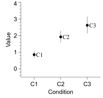
The figure is looking pretty good—let’s make a couple of final tweaks to finish it off. First, the labels attached to each point can be useful sometimes but are probably unnecessary here. Second, let’s add a white ring around each data point—mostly because it looks nice, but also to add a bit of separation between the point and its CI. Finally, let’s make the points a bit bigger.

import numpy as np
import scipy.stats

import veusz.embed

data_path = "prog_data_vis_descriptives_sim_data.tsv"

# load the data we generated in the previous step
data = np.loadtxt(data_path, delimiter="\t")

# pull out some design parameters from the shape of the array
n_per_group = data.shape[0]
n_cond = data.shape[1]
subjects = range(n_per_group)

embed = veusz.embed.Embedded("veusz")

page = embed.Root.Add("page")
page.width.val = "8.4cm"
page.height.val = "8cm"

graph = page.Add("graph", autoadd=False)

x_axis = graph.Add("axis")
y_axis = graph.Add("axis")

n_boot = 10000

cond_labels = ["C1", "C2", "C3"]

for i_cond in range(n_cond):

    cond_mean = np.mean(data[:, i_cond])

    # do bootstrapping
    boot_data = np.empty(n_boot)
    boot_data.fill(np.nan)

    for i_boot in range(n_boot):

        rand_subj_sample = np.random.choice(
            a=subjects,
            replace=True,
            size=n_per_group
        )

        boot_data[i_boot] = np.mean(data[rand_subj_sample, i_cond])

    lower_ci = scipy.stats.scoreatpercentile(boot_data, 2.5)
    upper_ci = scipy.stats.scoreatpercentile(boot_data, 97.5)

    pos_err = upper_ci - cond_mean
    neg_err = lower_ci - cond_mean

    data_str = "cond_{i:d}".format(i=i_cond)

    # cond_mean is a single value whereas SetData is expecting a list or array,
    # so pass a one-item list
    embed.SetData(
        data_str,
        [cond_mean],
        poserr=[pos_err],
        negerr=[neg_err]
    )

    xy = graph.Add("xy")

    xy.xData.val = i_cond
    xy.yData.val = data_str
    xy.labels.val = cond_labels[i_cond]

    xy.Label.hide.val = True
    xy.MarkerLine.color.val = "white"
    xy.MarkerLine.width.val = "2pt"

    xy.markerSize.val = "4pt"

x_axis.mode.val = "labels"
x_axis.MajorTicks.manualTicks.val = range(n_cond)
x_axis.MinorTicks.hide.val = True
x_axis.label.val = "Condition"
x_axis.min.val = -0.5
x_axis.max.val = 2.5

y_axis.min.val = -0.5
y_axis.max.val = 4.0
y_axis.label.val = "Value"

# do the typical manipulations to the axis apperances
graph.Border.hide.val = True

typeface = "Arial"

for curr_axis in [x_axis, y_axis]:

    curr_axis.Label.font.val = typeface
    curr_axis.TickLabels.font.val = typeface

    curr_axis.autoMirror.val = False
    curr_axis.outerticks.val = True

embed.WaitForClose()