Experimental design—power analysis and its visualisation

Objectives

• Be able to perform power calculations using computational simulation approaches.
• Know how to create and use line and image plots.

Power relates to the ability to detect the presence of a true effect and is an important component of experimental design. In this lesson, we will consider a general-purpose simulation approach to estimating the power of an experimental design. We will also investigate how we can visualise such data using line plots and two-dimensional image plots.

Calculating power given effect size and sample size

We will begin by considering a scenario in which we have an effect size and sample size in mind and we would like to know the associated power. For our example experiment, we will use a between-subjects design with two factors, 30 participants per group, and we will assume a ‘large’ effect size (Cohen’s d = 0.8). You might recognise this design, as it was the same that we used in the previous lesson to demonstrate the operation of the independent-samples t-test. Here, we will determine the power of this test.

The key to determining power using a simulation approach is to again leverage the computational capacity that we have once we are able to write our own programs. We will perform a large number of simulated experiments, each time calculating our test statistic (independent samples t-test, in this case) and accumulating the number of times we reject the null hypothesis. Then, the power is simply the proportion of times that we are able to reject the null hypothesis (remembering that we control the population means and we know that there is a true difference).

import numpy as np

import scipy.stats

n_per_group = 30

# effect size = 0.8
group_means = [0.0, 0.8]
group_sigmas = [1.0, 1.0]

n_groups = len(group_means)

# number of simulations
n_sims = 10000

# store the p value for each simulation
sim_p = np.empty(n_sims)
sim_p.fill(np.nan)

for i_sim in range(n_sims):

    data = np.empty([n_per_group, n_groups])
    data.fill(np.nan)

    # simulate the data for this 'experiment'
    for i_group in range(n_groups):

        data[:, i_group] = np.random.normal(
            loc=group_means[i_group],
            scale=group_sigmas[i_group],
            size=n_per_group
        )

    result = scipy.stats.ttest_ind(data[:, 0], data[:, 1])

    sim_p[i_sim] = result[1]

# number of simulations where the null was rejected
n_rej = np.sum(sim_p < 0.05)

prop_rej = n_rej / float(n_sims)

print "Power: ", prop_rej

Power:  0.8619

We can see that our power to detect a large effect size with 30 participants per group in a between-subjects design is about 86%. That is, if a large effect size is truly present then we would expect to be able to reject the null hypothesis (at an alpha of 0.05) about 86% of the time.

The above code was written with clarity rather than speed of execution in mind, but in subsequent examples we would like to perform more computationally demanding analyses—so let’s make some tweaks to allow it to be performed quicker. In the code below, we generate the simulated data all at once and then use the axis argument to scipy.stats.ttest_ind.

import numpy as np

import scipy.stats

n_per_group = 30

# effect size = 0.8
group_means = [0.0, 0.8]
group_sigmas = [1.0, 1.0]

n_groups = len(group_means)

# number of simulations
n_sims = 10000

data = np.empty([n_sims, n_per_group, n_groups])
data.fill(np.nan)

for i_group in range(n_groups):

    data[:, :, i_group] = np.random.normal(
        loc=group_means[i_group],
        scale=group_sigmas[i_group],
        size=[n_sims, n_per_group]
    )

result = scipy.stats.ttest_ind(
    data[:, :, 0],
    data[:, :, 1],
    axis=1
)

sim_p = result[1]

# number of simulations where the null was rejected
n_rej = np.sum(sim_p < 0.05)

prop_rej = n_rej / float(n_sims)

print "Power: ", prop_rej

Power:  0.8596

Required sample size to achieve a given power for a given effect size

Now we will move on to a more common scenario, where you have a design and effect size in mind and would like to know what sample size you would need to achieve a particular power (80% is typical). This is a straightforward extension of the previous example: we begin with a sample size and calculate the associated power. We then perform such a calculation repeatedly, each time increasing the sample size, until the power has reached the desired level.

import numpy as np

import scipy.stats

# start at 20 participants
n_per_group = 20

# effect size = 0.8
group_means = [0.0, 0.8]
group_sigmas = [1.0, 1.0]

n_groups = len(group_means)

# number of simulations
n_sims = 10000

# power level that we would like to reach
desired_power = 0.8

# initialise the power for the current sample size to a small value
current_power = 0.0

# keep iterating until desired power is obtained
while current_power < desired_power:

    data = np.empty([n_sims, n_per_group, n_groups])
    data.fill(np.nan)

    for i_group in range(n_groups):

        data[:, :, i_group] = np.random.normal(
            loc=group_means[i_group],
            scale=group_sigmas[i_group],
            size=[n_sims, n_per_group]
        )

    result = scipy.stats.ttest_ind(
        data[:, :, 0],
        data[:, :, 1],
        axis=1
    )

    sim_p = result[1]

    # number of simulations where the null was rejected
    n_rej = np.sum(sim_p < 0.05)

    prop_rej = n_rej / float(n_sims)

    current_power = prop_rej

    print "With {n:d} samples per group, power = {p:.3f}".format(
        n=n_per_group,
        p=current_power
    )

    # increase the number of samples by one for the next iteration of the loop
    n_per_group += 1

With 20 samples per group, power = 0.697
With 21 samples per group, power = 0.714
With 22 samples per group, power = 0.738
With 23 samples per group, power = 0.755
With 24 samples per group, power = 0.769
With 25 samples per group, power = 0.791
With 26 samples per group, power = 0.801

We can see that we would reach the desired power with somewhere between 25 and 27 participants per group.

Visualising the sample size/power relationship

In the previous example, we sought to determine the sample size that would provide a given level of power. However, perhaps we do not have a single level of power in mind at the moment but would like to see the relationship between sample size and power so that we can see the costs and benefits of a particular sample size.

First, we will use a similar approach to the previous example, however we will perform the simulations across a fixed set of sample sizes. We will then save the power values to disk so that we can use them to create a visualisation without having to re-run all the simulations.

import numpy as np

import scipy.stats

# let's look at samples sizes of 10 per group up to 50 per group in steps of 5
ns_per_group = np.arange(10, 51, 5)

# a bit awkward - number of n's
n_ns = len(ns_per_group)

# effect size = 0.8
group_means = [0.0, 0.8]
group_sigmas = [1.0, 1.0]

n_groups = len(group_means)

# number of simulations
n_sims = 10000

power = np.empty(n_ns)
power.fill(np.nan)

for i_n in range(n_ns):

    n_per_group = ns_per_group[i_n]

    data = np.empty([n_sims, n_per_group, n_groups])
    data.fill(np.nan)

    for i_group in range(n_groups):

        data[:, :, i_group] = np.random.normal(
            loc=group_means[i_group],
            scale=group_sigmas[i_group],
            size=[n_sims, n_per_group]
        )

    result = scipy.stats.ttest_ind(
        data[:, :, 0],
        data[:, :, 1],
        axis=1
    )

    sim_p = result[1]

    # number of simulations where the null was rejected
    n_rej = np.sum(sim_p < 0.05)

    prop_rej = n_rej / float(n_sims)

    power[i_n] = prop_rej

# this is a bit tricky
# what we want to save is an array with 2 columns, but we have 2 different 1D
# arrays. here, we use the 'np.newaxis' property to add a column each of the
# two 1D arrays, and then 'stack' them horizontally
array_to_save = np.hstack(
    [
        ns_per_group[:, np.newaxis],
        power[:, np.newaxis]
    ]
)

power_path = "prog_data_vis_power_sim_data.tsv"

np.savetxt(
    power_path,
    array_to_save,
    delimiter="\t",
    header="Simulated power as a function of samples per group"
)

Now, we want to begin our visualisation code by loading the data we just saved.

import numpy as np

power_path = "prog_data_vis_power_sim_data.tsv"

power = np.loadtxt(power_path, delimiter="\t")

# number of n's is the number of rows
n_ns = power.shape[0]

ns_per_group = power[:, 0]
power_per_ns = power[:, 1]

We will now use familiar techniques to set up a one-panel figure. We will also apply some of the usual formatting changes.

import numpy as np

import veusz.embed

power_path = "prog_data_vis_power_sim_data.tsv"

power = np.loadtxt(power_path, delimiter="\t")

# number of n's is the number of rows
n_ns = power.shape[0]

ns_per_group = power[:, 0]
power_per_ns = power[:, 1]

embed = veusz.embed.Embedded("veusz")

page = embed.Root.Add("page")
page.width.val = "8.4cm"
page.height.val = "8cm"

graph = page.Add("graph", autoadd=False)

x_axis = graph.Add("axis")
y_axis = graph.Add("axis")


# do the typical manipulations to the axis apperances
graph.Border.hide.val = True

typeface = "Arial"

for curr_axis in [x_axis, y_axis]:

    curr_axis.Label.font.val = typeface
    curr_axis.TickLabels.font.val = typeface

    curr_axis.autoMirror.val = False
    curr_axis.outerticks.val = True

embed.WaitForClose()

Alright, now we can plot the sample size per group on the horizontal axis and the power on the vertical axis. We will use the familiar xy figure type.

import numpy as np

import veusz.embed

power_path = "prog_data_vis_power_sim_data.tsv"

power = np.loadtxt(power_path, delimiter="\t")

# number of n's is the number of rows
n_ns = power.shape[0]

ns_per_group = power[:, 0]
power_per_ns = power[:, 1]

embed = veusz.embed.Embedded("veusz")

page = embed.Root.Add("page")
page.width.val = "8.4cm"
page.height.val = "8cm"

graph = page.Add("graph", autoadd=False)

x_axis = graph.Add("axis")
y_axis = graph.Add("axis")

# let veusz know about the data
embed.SetData("ns_per_group", ns_per_group)
embed.SetData("power_per_ns", power_per_ns)

xy = graph.Add("xy")

xy.xData.val = "ns_per_group"
xy.yData.val = "power_per_ns"

# do the typical manipulations to the axis apperances
graph.Border.hide.val = True

typeface = "Arial"

for curr_axis in [x_axis, y_axis]:

    curr_axis.Label.font.val = typeface
    curr_axis.TickLabels.font.val = typeface

    curr_axis.autoMirror.val = False
    curr_axis.outerticks.val = True

embed.WaitForClose()

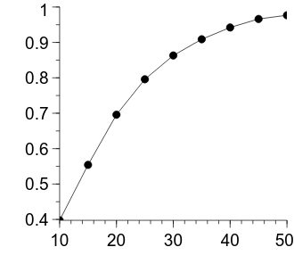
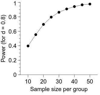
The figure is looking pretty good—the decelerating relationship between the number of samples in each group and the power is clearly evident. Let’s apply some more formatting changes to improve its appearance.

import numpy as np

import veusz.embed

power_path = "prog_data_vis_power_sim_data.tsv"

power = np.loadtxt(power_path, delimiter="\t")

# number of n's is the number of rows
n_ns = power.shape[0]

ns_per_group = power[:, 0]
power_per_ns = power[:, 1]

embed = veusz.embed.Embedded("veusz")

page = embed.Root.Add("page")
page.width.val = "8.4cm"
page.height.val = "8cm"

graph = page.Add("graph", autoadd=False)

x_axis = graph.Add("axis")
y_axis = graph.Add("axis")

# let veusz know about the data
embed.SetData("ns_per_group", ns_per_group)
embed.SetData("power_per_ns", power_per_ns)

xy = graph.Add("xy")

xy.xData.val = "ns_per_group"
xy.yData.val = "power_per_ns"

# set the x ticks to be at every 2nd location we sampled
x_axis.MajorTicks.manualTicks.val = ns_per_group[::2].tolist()
x_axis.MinorTicks.hide.val = True
x_axis.label.val = "Sample size per group"
x_axis.min.val = float(np.min(ns_per_group) - 5)
x_axis.max.val = float(np.max(ns_per_group) + 5)

# sensible to include the whole range here
y_axis.min.val = 0.0
y_axis.max.val = 1.0
y_axis.label.val = "Power (for d = 0.8)"

# do the typical manipulations to the axis apperances
graph.Border.hide.val = True

typeface = "Arial"

for curr_axis in [x_axis, y_axis]:

    curr_axis.Label.font.val = typeface
    curr_axis.TickLabels.font.val = typeface

    curr_axis.autoMirror.val = False
    curr_axis.outerticks.val = True

embed.WaitForClose()

Calculating power across varying sample and effect sizes

In the previous examples, we have assumed a fixed (‘large’) effect size. However, perhaps we want to investigate how power changes with both effect size and sample size. This is again a straightforward extension of the previous example. We will again save the data to disk to facilitate subsequent visualisation.

import numpy as np

import scipy.stats

# let's look at samples sizes of 10 per group up to 50 per group in steps of 5
ns_per_group = np.arange(10, 51, 5)

# a bit awkward - number of n's
n_ns = len(ns_per_group)

# span the range from a bit less than a 'small' effect size to a bit bigger
# than a 'large' effect size
effect_sizes = np.arange(0.2, 0.91, 0.1)

n_effect_sizes = len(effect_sizes)

power = np.empty([n_effect_sizes, n_ns])
power.fill(np.nan)

# number of simulations
n_sims = 10000

for i_es in range(n_effect_sizes):

    group_means = [0.0, effect_sizes[i_es]]
    group_sigmas = [1.0, 1.0]

    n_groups = len(group_means)

    for i_n in range(n_ns):

        n_per_group = ns_per_group[i_n]

        data = np.empty([n_sims, n_per_group, n_groups])
        data.fill(np.nan)

        for i_group in range(n_groups):

            data[:, :, i_group] = np.random.normal(
                loc=group_means[i_group],
                scale=group_sigmas[i_group],
                size=[n_sims, n_per_group]
            )

        result = scipy.stats.ttest_ind(
            data[:, :, 0],
            data[:, :, 1],
            axis=1
        )

        sim_p = result[1]

        # number of simulations where the null was rejected
        n_rej = np.sum(sim_p < 0.05)

        prop_rej = n_rej / float(n_sims)

        power[i_es, i_n] = prop_rej

power_path = "prog_data_vis_power_es_x_ss_sim_data.tsv"

np.savetxt(
    power_path,
    power,
    delimiter="\t",
    header="Simulated power as a function of samples per group and ES"
)

Visualising power across varying sample and effect sizes

Now that we have our power calculations as a function of sample size and effect size saved to disk, we can think about how to visualise it. But first, let’s load the data.

import numpy as np

power_path = "prog_data_vis_power_es_x_ss_sim_data.tsv"

power = np.loadtxt(power_path, delimiter="\t")

# number of effect sizes is the number of rows
n_effect_sizes = power.shape[0]
# number of n's is the number of columns
n_ns = power.shape[1]

ns_per_group = np.arange(10, 51, 5)
effect_sizes = np.arange(0.2, 0.91, 0.1)

To visualise this two-dimensional data (effect size x sample size per group), we will investigate a new veusz figure type—an image. First, let’s set up our figure framework as per usual.

import numpy as np

import veusz.embed

power_path = "prog_data_vis_power_es_x_ss_sim_data.tsv"

power = np.loadtxt(power_path, delimiter="\t")

# number of effect sizes is the number of rows
n_effect_sizes = power.shape[0]
# number of n's is the number of columns
n_ns = power.shape[1]

ns_per_group = np.arange(10, 51, 5)
effect_sizes = np.arange(0.2, 0.91, 0.1)

embed = veusz.embed.Embedded("veusz")

page = embed.Root.Add("page")
page.width.val = "8.4cm"
page.height.val = "8cm"

graph = page.Add("graph", autoadd=False)

x_axis = graph.Add("axis")
y_axis = graph.Add("axis")

# do the typical manipulations to the axis apperances
graph.Border.hide.val = True

typeface = "Arial"

for curr_axis in [x_axis, y_axis]:

    curr_axis.Label.font.val = typeface
    curr_axis.TickLabels.font.val = typeface

    curr_axis.autoMirror.val = False
    curr_axis.outerticks.val = True

embed.WaitForClose()

Now, we will add our image figure type to the graph. First, we tell veusz about the data using the SetData2D function, using the arguments xcent and ycent to tell veusz what the horizontal and vertical datapoints represent.

import numpy as np

import veusz.embed

power_path = "prog_data_vis_power_es_x_ss_sim_data.tsv"

power = np.loadtxt(power_path, delimiter="\t")

# number of effect sizes is the number of rows
n_effect_sizes = power.shape[0]
# number of n's is the number of columns
n_ns = power.shape[1]

ns_per_group = np.arange(10, 51, 5)
effect_sizes = np.arange(0.2, 0.91, 0.1)

embed = veusz.embed.Embedded("veusz")

page = embed.Root.Add("page")
page.width.val = "8.4cm"
page.height.val = "8cm"

graph = page.Add("graph", autoadd=False)

x_axis = graph.Add("axis")
y_axis = graph.Add("axis")

embed.SetData2D(
    "power",
    power,
    xcent=ns_per_group,
    ycent=effect_sizes
)

img = graph.Add("image")

img.data.val = "power"

# do the typical manipulations to the axis apperances
graph.Border.hide.val = True

typeface = "Arial"

for curr_axis in [x_axis, y_axis]:

    curr_axis.Label.font.val = typeface
    curr_axis.TickLabels.font.val = typeface

    curr_axis.autoMirror.val = False
    curr_axis.outerticks.val = True

embed.WaitForClose()

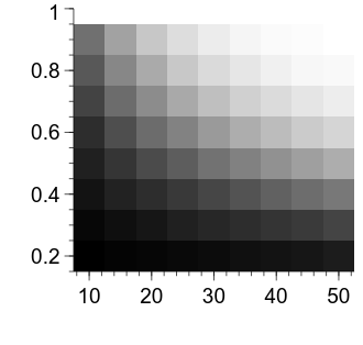
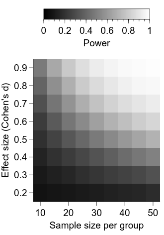
Now we are starting to get somewhere—we can see that the power for a given combination of effect size and sample size per group is represented by the luminance of the relevant cell. Let’s first clean up the appearance of the figure a bit.

import numpy as np

import veusz.embed

power_path = "prog_data_vis_power_es_x_ss_sim_data.tsv"

power = np.loadtxt(power_path, delimiter="\t")

# number of effect sizes is the number of rows
n_effect_sizes = power.shape[0]
# number of n's is the number of columns
n_ns = power.shape[1]

ns_per_group = np.arange(10, 51, 5)
effect_sizes = np.arange(0.2, 0.91, 0.1)

embed = veusz.embed.Embedded("veusz")

page = embed.Root.Add("page")
page.width.val = "8.4cm"
page.height.val = "8cm"

graph = page.Add("graph", autoadd=False)

x_axis = graph.Add("axis")
y_axis = graph.Add("axis")

embed.SetData2D(
    "power",
    power,
    xcent=ns_per_group,
    ycent=effect_sizes
)

img = graph.Add("image")

img.data.val = "power"

# set 0.0 = black and 1.0 = white
img.min.val = 0.0
img.max.val = 1.0

x_axis.MajorTicks.manualTicks.val = ns_per_group[::2].tolist()
x_axis.MinorTicks.hide.val = True
x_axis.label.val = "Sample size per group"

y_axis.MajorTicks.manualTicks.val = effect_sizes.tolist()
y_axis.MinorTicks.hide.val = True
y_axis.label.val = "Effect size (Cohen's d)"
y_axis.max.val = float(np.max(effect_sizes) + 0.05)

# do the typical manipulations to the axis apperances
graph.Border.hide.val = True

typeface = "Arial"

for curr_axis in [x_axis, y_axis]:

    curr_axis.Label.font.val = typeface
    curr_axis.TickLabels.font.val = typeface

    curr_axis.autoMirror.val = False
    curr_axis.outerticks.val = True

embed.WaitForClose()

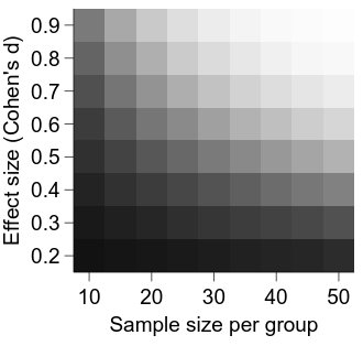
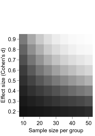
It is looking better, but a major deficiency at the moment is a lack of information about what the intensity in each cell represents. To remedy this, we will add a colorbar to our graph. But first, we will make room for it by increasing our vertical page size and increasing the top margin of our graph.

import numpy as np

import veusz.embed

power_path = "prog_data_vis_power_es_x_ss_sim_data.tsv"

power = np.loadtxt(power_path, delimiter="\t")

# number of effect sizes is the number of rows
n_effect_sizes = power.shape[0]
# number of n's is the number of columns
n_ns = power.shape[1]

ns_per_group = np.arange(10, 51, 5)
effect_sizes = np.arange(0.2, 0.91, 0.1)

embed = veusz.embed.Embedded("veusz")

page = embed.Root.Add("page")
page.width.val = "8.4cm"
page.height.val = "12cm"

graph = page.Add("graph", autoadd=False)

graph.topMargin.val = "3cm"

x_axis = graph.Add("axis")
y_axis = graph.Add("axis")

embed.SetData2D(
    "power",
    power,
    xcent=ns_per_group,
    ycent=effect_sizes
)

img = graph.Add("image")

img.data.val = "power"

# set 0.0 = black and 1.0 = white
img.min.val = 0.0
img.max.val = 1.0

x_axis.MajorTicks.manualTicks.val = ns_per_group[::2].tolist()
x_axis.MinorTicks.hide.val = True
x_axis.label.val = "Sample size per group"

y_axis.MajorTicks.manualTicks.val = effect_sizes.tolist()
y_axis.MinorTicks.hide.val = True
y_axis.label.val = "Effect size (Cohen's d)"
y_axis.max.val = float(np.max(effect_sizes) + 0.05)

# do the typical manipulations to the axis apperances
graph.Border.hide.val = True

typeface = "Arial"

for curr_axis in [x_axis, y_axis]:

    curr_axis.Label.font.val = typeface
    curr_axis.TickLabels.font.val = typeface

    curr_axis.autoMirror.val = False
    curr_axis.outerticks.val = True

embed.WaitForClose()

Now, we can add and position the colour bar:

import numpy as np

import veusz.embed

power_path = "prog_data_vis_power_es_x_ss_sim_data.tsv"

power = np.loadtxt(power_path, delimiter="\t")

# number of effect sizes is the number of rows
n_effect_sizes = power.shape[0]
# number of n's is the number of columns
n_ns = power.shape[1]

ns_per_group = np.arange(10, 51, 5)
effect_sizes = np.arange(0.2, 0.91, 0.1)

embed = veusz.embed.Embedded("veusz")

page = embed.Root.Add("page")
page.width.val = "8.4cm"
page.height.val = "12cm"

graph = page.Add("graph", autoadd=False)

graph.topMargin.val = "3cm"

x_axis = graph.Add("axis")
y_axis = graph.Add("axis")

embed.SetData2D(
    "power",
    power,
    xcent=ns_per_group,
    ycent=effect_sizes
)

# give the image a 'name', so that we can tell the colour bar what image it
# should be associated with
img = graph.Add("image", name="power_img")

img.data.val = "power"

# set 0.0 = black and 1.0 = white
img.min.val = 0.0
img.max.val = 1.0

cbar = graph.Add("colorbar")

# connect the colour bar with the power image
cbar.widgetName.val = "power_img"
cbar.horzPosn.val = "centre"
cbar.vertPosn.val = "manual"
cbar.vertManual.val = -0.35
cbar.label.val = "Power"

x_axis.MajorTicks.manualTicks.val = ns_per_group[::2].tolist()
x_axis.MinorTicks.hide.val = True
x_axis.label.val = "Sample size per group"

y_axis.MajorTicks.manualTicks.val = effect_sizes.tolist()
y_axis.MinorTicks.hide.val = True
y_axis.label.val = "Effect size (Cohen's d)"
y_axis.max.val = float(np.max(effect_sizes) + 0.05)

# do the typical manipulations to the axis apperances
graph.Border.hide.val = True

typeface = "Arial"

for curr_axis in [x_axis, y_axis, cbar]:

    curr_axis.Label.font.val = typeface
    curr_axis.TickLabels.font.val = typeface

    curr_axis.autoMirror.val = False
    curr_axis.outerticks.val = True

embed.WaitForClose()