Rendering stimuli for perception studies using Mitsuba 2

2020-Jul-02

Realistic three-dimensional rendering is useful for running and interpreting perception studies. Here, I describe using the Python interface to the Mitsuba 2 physically-based renderer to reproduce the key aspects of the stimuli from a published article in perception.

I am currently teaching a seminar on “Illumination and human vision” in which we consider a range of studies that investigate how illumination is treated by the human visual system. As part of the seminar, we have been exploring the computer graphics aspect of stimulus generation. This perspective adds a practical component to the seminar, but also shifts the focus away from just images and towards the environmental components that come together to form images.

We considered the stimuli in the neat study by Snyder, Doerschner, & Maloney (2005) as an example. We used the three.js editor to explore the scene interactively in a web browser and see it rendered with approximations that permitted real-time rendering. However, these rendering limitations meant that we couldn’t reproduce many important aspects of the stimuli used in the study.

This gave me a chance to try out the newly-released version 2 of Mitsuba, which is one of my favourite pieces of software. Mitsuba is a physically-based renderer that takes in a textual description of a scene and produces beautifully realistic images. I find describing a scene in text rather than via a graphical interface to be much more intuitive and suitable for stimulus generation purposes. Mitsuba also has the best documentation of any software I have come across and is also wonderful for learning about the broader issues involved in image formation.

Here, I’m going to walk through my recreation of something similar to the stimulus in Snyder, Doerschner, & Maloney (2005). I’ll use the direct Python interface to Mitsuba, rather than using Python to generate the scene description and provide it to the mitsuba binary (which I did previously in 3D Rendering With Mitsuba).

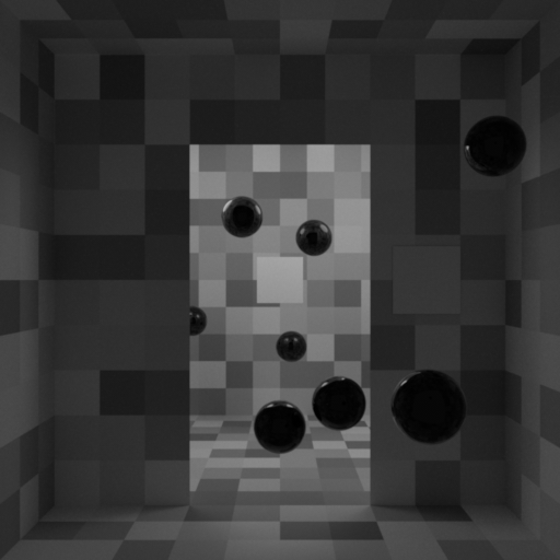
We will end up producing this image:

Rendering of a room with checkerboard walls and floating mirror-reflective spheres — Rendering of a stimulus similar to that used in Snyder, Doerschner, & Maloney (2005), produced using Mitsuba 2.

I’ll be walking through snippets of code that implement different aspects of functionality—these snippets should be thought of as successive chunks of code. Note that the code will be written more for ease of exposition than for good coding practices. I also won’t be going into too much detail on why many components are structured how they are—see the Mitsuba documentation for the specific details.

Importing

The first step is to import Mitsuba and the other packages we will need. Because version 2 of Mitsuba can be compiled with the potential to render with multiple variants, we need to tell mitsuba which one we want to use immediately after it is imported.

import mitsuba
mitsuba.set_variant(value="scalar_rgb")

We will also need numpy, so we import it here. To have reproducible randomness, we also create a random state with a fixed seed (one that gave a good set of sphere positions).

import numpy as np
random = np.random.RandomState(seed=19)

Finally, we will use imageio to save the rendering (and some intermediate textures).

import imageio

Geometry

We will start our scene description with its geometry. First, we will specify the layout of the room (walls, floor, and ceiling) and the two ‘patches’ (standard and comparison). Then, we will add the set of spheres.

To begin, we create some variables that specify the dimensions of the room; 5 units wide, 5 units high, and 10 units deep.

room_width = 5
room_halfwidth = room_width / 2

room_height = 5
room_halfheight = room_height / 2

room_depth = 10
room_halfdepth = room_depth / 2

Next, we define a helper variable that specifies the axis vectors. This will assist when orienting the surfaces.

(x, y, z) = ((1, 0, 0), (0, 1, 0), (0, 0, 1))

Not all of the surfaces will need rotating about their default orientations, so we create another helper variable that specifies a null rotation.

null_rotation = {"axis": x, "angle": 0}

Our approach will be to use a set of planes to specify the surface geometry, each created as a rectangle shape. The default is for the plane to cover from [-1, -1, 0] to [+1, +1, 0]; we apply a translation, rotation, and scaling transformation to position it correctly in our scene. First, we specify the required transformations of each of the room planes in a dict; note that this is just for our organisation and is not related to Mitsuba yet.

surface_transforms = {
    "floor": {
        "scale": (room_halfwidth, room_halfdepth),
        "rotation": {"axis": x, "angle": -90},
        "translation": (0, -room_halfwidth, -room_halfdepth),
    },
    "roof": {
        "scale": (room_halfwidth, room_halfdepth),
        "rotation": {"axis": x, "angle": 90},
        "translation": (0, room_halfwidth, -room_halfdepth),
    },
    "back": {
        "scale": (room_halfwidth, room_halfheight),
        "rotation": null_rotation,
        "translation": (0, 0, -room_depth),
    },
    "left": {
        "scale": (room_halfdepth, room_halfheight),
        "rotation": {"axis": y, "angle": 90},
        "translation": (-room_halfwidth, 0, -room_halfdepth),
    },
    "right": {
        "scale": (room_halfdepth, room_halfheight),
        "rotation": {"axis": y, "angle": -90},
        "translation": (room_halfwidth, 0, -room_halfdepth),
    },
    "mid_left": {
        "scale": (room_halfwidth * 0.3, room_halfheight),
        "rotation": null_rotation,
        "translation": (room_halfwidth * 0.3 - room_halfwidth, 0, -room_halfdepth),
    },
    "mid_right": {
        "scale": (room_halfwidth * 0.3, room_halfheight),
        "rotation": null_rotation,
        "translation": (room_halfwidth * 0.7, 0, -room_halfdepth),
    },
    "mid_top": {
        "scale": (room_halfwidth * 0.4, room_halfheight * 0.2),
        "rotation": null_rotation,
        "translation": (0, room_halfheight * 0.8, -room_halfdepth),
    },
}

Let’s do the same thing for the comparison surface.

surface_transforms["comparison"] = {
    "scale": (room_halfwidth * 0.3 / 2,) * 2,
    "rotation": null_rotation,
    "translation": (room_halfwidth * 0.65, 0, -room_halfdepth + 0.01),
}

The standard surface is presented at different distances in their study; here, let’s put it towards the far wall.

standard_depth = 8.5

surface_transforms["standard"] = {
    "scale": surface_transforms["comparison"]["scale"],
    "rotation": null_rotation,
    "translation": (0, 0, -standard_depth),
}

Now that we have all of our transformations sorted out, we can assemble the set of surfaces in Mitsuba format.

surfaces = {
    surface_name: {
        "type": "rectangle",
        "to_world": (
            mitsuba.core.Transform4f.translate(v=surface["translation"])
            * mitsuba.core.Transform4f.rotate(
                axis=surface["rotation"]["axis"], angle=surface["rotation"]["angle"]
            )
            * mitsuba.core.Transform4f.scale(v=surface["scale"] + (1,))
        ),
    }
    for (surface_name, surface) in surface_transforms.items()
}

Next, we want to add the spheres into the scene. Let’s first set some of the sphere properties.

n_spheres = 10
sphere_r = 0.25
sphere_d = sphere_r * 2

Now, we generate their random (well, sort of random given the use of a fixed seed) positions within the room.

sphere_positions = random.uniform(
    low=(
        -room_halfwidth + sphere_d,
        -room_halfheight + sphere_d,
        -room_depth + sphere_d,
    ),
    high=(room_halfwidth - sphere_d, room_halfheight - sphere_d, sphere_d * 2),
    size=(n_spheres, 3),
)

Then, we specify the spheres using the Mitsuba sphere shape.

spheres = {
    f"sphere{sphere_num:d}": {
        "type": "sphere",
        "center": sphere_position,
        "radius": sphere_r,
    }
    for (sphere_num, sphere_position) in enumerate(sphere_positions, 1)
}

Since we are using Python version 3.8, which does not yet have union operators for dictionaries, we use the update method of our surfaces dictionary to include the spheres.

surfaces.update(spheres)

That completes our specification of the scene geometry.

Materials

Now that we’ve specified where the surfaces will reside, we need to specify their material properties.

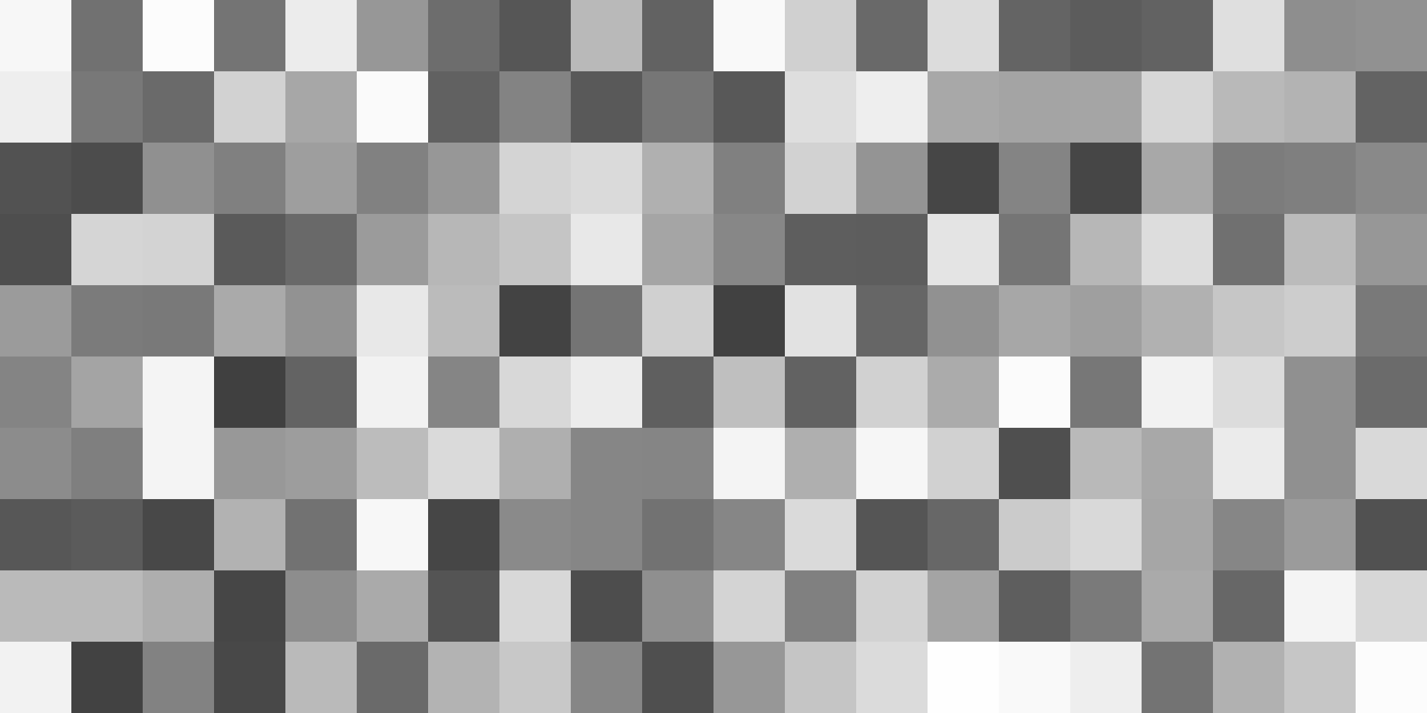
We will start with the room surfaces, which each have checkerboard-style surface reflectance. Each check is 0.5 units in size.

check_size = 0.5

To specify the checks, we will generate an image that we can apply as a texture to the surface. We could usually do that with one pixel per check, but Mitsuba does not (yet?) support nearest-neighbour texture interpolation. Instead, we upsample the texture by a specified factor.

check_upsample_factor = 100

Here, we will generate the textures for each of the room surfaces by drawing random reflectances and saving as an 8-bit PNG file.

for (surface_name, surface) in surfaces.items():

    if surface_name in ["comparison", "standard"] or surface_name.startswith("sphere"):
        continue

    surface_scale = np.array(surface_transforms[surface_name]["scale"])

    surface_size = surface_scale * 2

    n_checks = (surface_size / check_size).astype("int")

    checks = random.uniform(low=0.25, high=1.0, size=n_checks[::-1])

    texture = np.around(checks * 255).astype("uint8")

    texture = np.repeat(
        np.repeat(texture, repeats=check_upsample_factor, axis=0),
        repeats=check_upsample_factor,
        axis=1,
    )

    texture_path = surface_name + "_texture.png"

    imageio.imsave(texture_path, texture)

Here’s what one of the textures looks like.

Example checkerboard texture that is mapped to a wall in the room.

Now, we specify the texture path as the source of the reflectance properties of a diffuse (Lambertian) BRDF.

Because we are still operating within the loop opened above, I will reproduce the previous chunk below and highlight the added lines.

for (surface_name, surface) in surfaces.items():

    if surface_name in ["comparison", "standard"] or surface_name.startswith("sphere"):
        continue

    surface_scale = np.array(surface_transforms[surface_name]["scale"])

    surface_size = surface_scale * 2

    n_checks = (surface_size / check_size).astype("int")

    checks = random.uniform(low=0.25, high=1.0, size=n_checks[::-1])

    texture = np.around(checks * 255).astype("uint8")

    texture = np.repeat(
        np.repeat(texture, repeats=check_upsample_factor, axis=0),
        repeats=check_upsample_factor,
        axis=1,
    )

    texture_path = surface_name + "_texture.png"

    imageio.imsave(texture_path, texture)

    surface["material"] = {
        "type": "diffuse",
        "reflectance": {"type": "bitmap", "filename": texture_path, "raw": True},
    }

Finally, we need to account for the fact that three of our surfaces (the ‘mid’ surfaces) are double-sided. We do this by nesting its material specification inside a twosided adapter.

for (surface_name, surface) in surfaces.items():

    if surface_name in ["comparison", "standard"] or surface_name.startswith("sphere"):
        continue

    surface_scale = np.array(surface_transforms[surface_name]["scale"])

    surface_size = surface_scale * 2

    n_checks = (surface_size / check_size).astype("int")

    checks = random.uniform(low=0.25, high=1.0, size=n_checks[::-1])

    texture = np.around(checks * 255).astype("uint8")

    texture = np.repeat(
        np.repeat(texture, repeats=check_upsample_factor, axis=0),
        repeats=check_upsample_factor,
        axis=1,
    )

    texture_path = surface_name + "_texture.png"

    imageio.imsave(texture_path, texture)

    surface["material"] = {
        "type": "diffuse",
        "reflectance": {"type": "bitmap", "filename": texture_path, "raw": True},
    }

    if "mid" in surface_name:
        surface["material"] = {
            "type": "twosided",
            "reflectance": surface["material"],
        }

Now we can move on to the two patches, which have straightforward constant reflectance values.

for (surface_name, surface) in surfaces.items():

    if surface_name not in ["comparison", "standard"]:
        continue

    surface["material"] = {
        "type": "diffuse",
        "reflectance": {"type": "spectrum", "value": 1.0},
    }

Finally, we have the spheres. These surfaces will have a plastic BRDF, with no diffuse reflectance.

for (surface_name, surface) in surfaces.items():

    if not surface_name.startswith("sphere"):
        continue

    surface["material"] = {"type": "plastic", "diffuse_reflectance": 0.0}

Lights

Next we have the light sources. We will have three sources in this scene: two area lights positioned behind the mid walls and an ambient-like light.

The area lights are instantiated by designating a sphere shape as an area emitter.

light_r = 0.625
light_strength = 3.0

lights = {
    f"{side:s}_light": {
        "type": "sphere",
        "center": [
            (room_halfwidth - light_r) * side_sign,
            room_halfwidth - light_r,
            -room_halfdepth - light_r - 1,
        ],
        "radius": light_r,
        "light": {
            "type": "area",
            "radiance": {"type": "spectrum", "value": light_strength},
        },
    }
    for (side, side_sign) in zip(["left", "right"], [-1, +1])
}

Next, we implement the ambient-like light via a constant emitter.

ambient_strength = 0.05

lights["ambient"] = {
    "type": "constant",
    "radiance": ambient_strength,
}

Camera

Now we have our surface geometry and materials and have specified the lighting, we can describe the camera as a perspective sensor.

camera = {
    "type": "perspective",
    "to_world": mitsuba.core.Transform4f.look_at(
        origin=(0, 0, room_halfheight), target=(0, 0, -room_depth), up=(0, 1, 0),
    ),
    "fov": 45.0,
}

We need to load some film into the camera, which we do by adding hdrfilm.

camera["film"] = {
    "type": "hdrfilm",
    "pixel_format": "luminance",
    "width": 512,
    "height": 512,
}

Next, we need to specify the type of sampler to use and its sample count. The sample count correlates with the ‘quality’ of the rendering, and also with the time taken to finish the render. Here, we will set it to a reasonably high value; it produces a nice-looking render in about 8 minutes on my machine.

camera["sampler"] = {"type": "independent", "sample_count": 4096}

Integrator

Finally, we specify a path tracer as the integrator. The max_depth parameter is useful for producing renders without mutual illumination; here, we want mutual illumination.

integrator = {"type": "path", "max_depth": -1}

Conversion to Mitsuba format

At this point, we have built up all our scene information in the surfaces, lights, camera, and integrator dictionaries. Now, we combine them together into a single scene dictionary.

scene = {"type": "scene", "camera": camera, "integrator": integrator}
scene.update(surfaces)
scene.update(lights)

We then provide it to Mitsuba to be parsed into its internal scene description.

mitsuba_scene = mitsuba.core.xml.load_dict(scene)

Rendering

Now we can extract some of the Mitsuba objects that we need for rendering from this Mitsuba scene representation.

(sensor,) = mitsuba_scene.sensors()
integrator = mitsuba_scene.integrator()

Now we can actually do the rendering!

integrator.render(scene=mitsuba_scene, sensor=sensor)

Next, we convert this raw rendering information into an array of 8-bit integers that represents the luminance in an sRGB colour space.

image = (
    sensor.film()
    .bitmap(raw=True)
    .convert(
        pixel_format=mitsuba.core.Bitmap.PixelFormat.Y,
        component_format=mitsuba.core.Struct.Type.UInt8,
        srgb_gamma=True,
    )
)

Finally, we save the array to a PNG file and we’re done!

image.write("snyder_scene_demo_render.png")

Summary

Here, we have used the Python interface to Mitsuba 2 to describe the structure of a three-dimensional scene and to render it to an image. This allowed us to replicate the key aspects of the stimuli used in the paper by Snyder, Doerschner, & Maloney (2005).

Here is the complete code file.

References

Snyder, J.L., Doerschner, K., & Maloney, L.T. (2005) Illumination estimation in three-dimensional scenes with and without specular cues. Journal of Vision, 5(10), 863–877.